SIRS Autonomous Model with Time-Dependent Parameters
This notebook explores the dynamics of a SIRS model with time-dependent infection and immunity waning rates:
\(\beta(t)\) models seasonal or serotype-driven infection rate
\(\alpha(t)\) models waning immunity dynamics
We simulate different epidemiological scenarios and analyze:
Infection waves
Endemic behavior
Effective reproduction number \(R_t\)
The model is motivated by dengue dynamics with alternating serotype dominance.
[1]:
import numpy as np
import matplotlib.pyplot as plt
from scipy.integrate import solve_ivp
[2]:
# Base parameters
rho_0 = 0.01
B_0 = 0.05

rho = np.array([0.05, 0.15, 0.10])
T = np.array([30.5, 82.5, 144.5])

B = np.array([0.4, 0.4, 0.35])
tau = np.array([12, 64, 123])

sigma = np.array([3.2, 3.2, 2.0])
sk = np.array([0.25, 0.25, 0.15])

gamma = 0.15
iota = 3
[3]:
def alpha(t):
    result = 0
    for i in range(len(rho)):
        result += rho[i] * ((1 + np.tanh(t - (T[i] - iota/2)))/2) * ((1 - np.tanh(t - (T[i] + iota/2)))/2)
    return rho_0 + result


def beta(t):
    result = 0
    for i in range(len(B)):
        result += B[i] * np.exp(-0.5 * ((t - tau[i]) / (sigma[i] + sk[i] * (t - tau[i])))**2)
    return B_0 + result


def Rt(t):
    return beta(t) / gamma
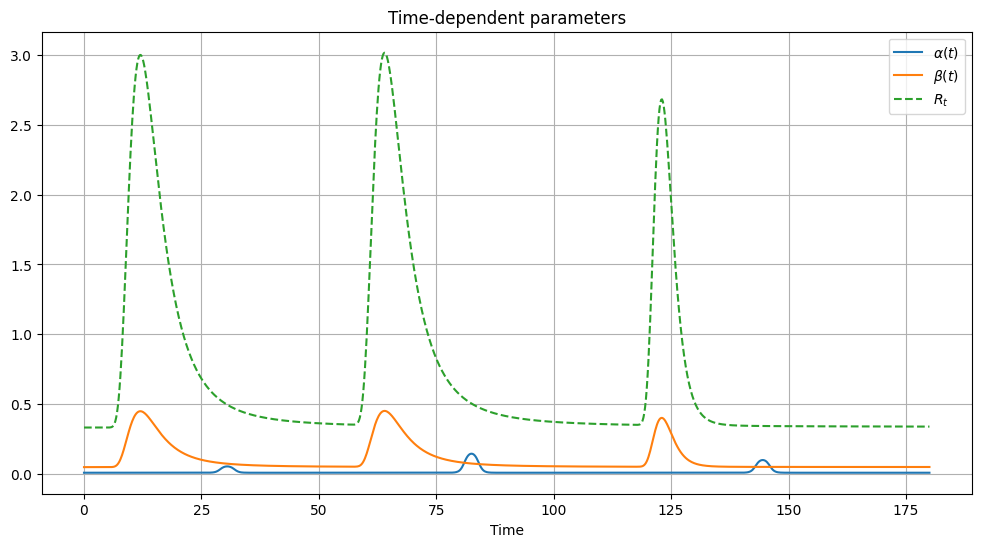
[4]:
t = np.linspace(0, 180, 1000)

plt.figure(figsize=(12, 6))
plt.plot(t, alpha(t), label=r'$\alpha(t)$')
plt.plot(t, beta(t), label=r'$\beta(t)$')
plt.plot(t, Rt(t), label=r'$R_t$', linestyle='--')
plt.legend()
plt.title("Time-dependent parameters")
plt.xlabel("Time")
plt.grid()
plt.show()
[5]:
def sirs_model(t, y):
    S, I, R = y

    dSdt = -beta(t) * S * I + alpha(t) * R
    dIdt = beta(t) * S * I - gamma * I
    dRdt = gamma * I - alpha(t) * R

    return [dSdt, dIdt, dRdt]
[6]:
# Initial conditions
S0 = 0.99
I0 = 0.01
R0 = 0.0

y0 = [S0, I0, R0]

t_span = (0, 180)
t_eval = np.linspace(*t_span, 1000)

sol = solve_ivp(sirs_model, t_span, y0, t_eval=t_eval)
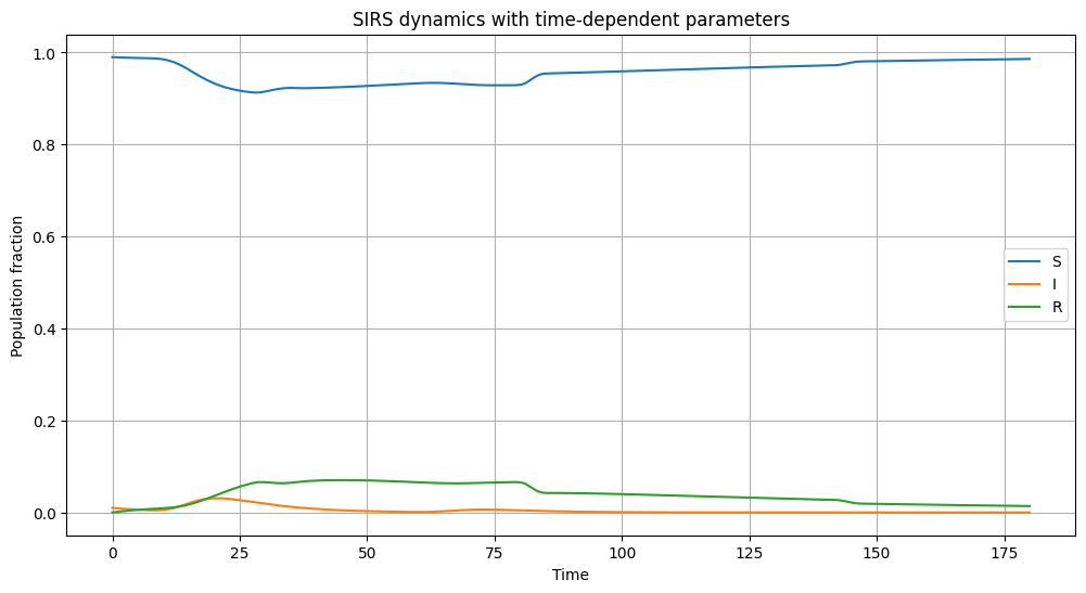
[7]:
plt.figure(figsize=(12, 6))
plt.plot(sol.t, sol.y[0], label='S')
plt.plot(sol.t, sol.y[1], label='I')
plt.plot(sol.t, sol.y[2], label='R')

plt.title("SIRS dynamics with time-dependent parameters")
plt.xlabel("Time")
plt.ylabel("Population fraction")
plt.legend()
plt.grid()
plt.show()
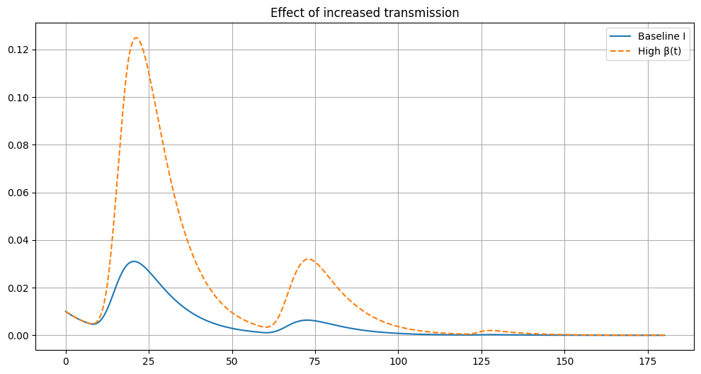
[8]:
B_high = B * 1.5

def beta_high(t):
    result = 0
    for i in range(len(B_high)):
        result += B_high[i] * np.exp(-0.5 * ((t - tau[i]) / (sigma[i] + sk[i] * (t - tau[i])))**2)
    return B_0 + result


def sirs_high(t, y):
    S, I, R = y
    return [
        -beta_high(t) * S * I + alpha(t) * R,
        beta_high(t) * S * I - gamma * I,
        gamma * I - alpha(t) * R
    ]

sol_high = solve_ivp(sirs_high, t_span, y0, t_eval=t_eval)

plt.figure(figsize=(12, 6))
plt.plot(sol.t, sol.y[1], label="Baseline I")
plt.plot(sol_high.t, sol_high.y[1], label="High β(t)", linestyle='--')
plt.legend()
plt.title("Effect of increased transmission")
plt.grid()
plt.show()
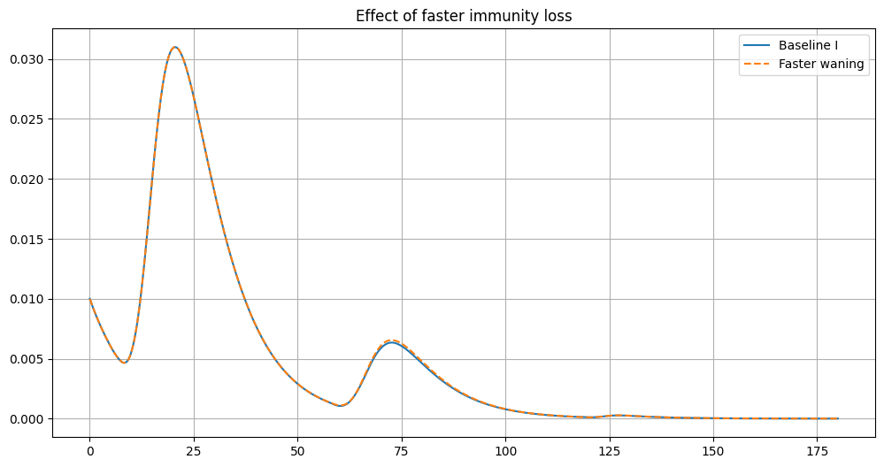
[9]:
rho_fast = rho * 1.5

def alpha_fast(t):
    result = 0
    for i in range(len(rho_fast)):
        result += rho_fast[i] * ((1 + np.tanh(t - (T[i] - iota/2)))/2) * ((1 - np.tanh(t - (T[i] + iota/2)))/2)
    return rho_0 + result


def sirs_fast(t, y):
    S, I, R = y
    return [
        -beta(t) * S * I + alpha_fast(t) * R,
        beta(t) * S * I - gamma * I,
        gamma * I - alpha_fast(t) * R
    ]

sol_fast = solve_ivp(sirs_fast, t_span, y0, t_eval=t_eval)

plt.figure(figsize=(12, 6))
plt.plot(sol.t, sol.y[1], label="Baseline I")
plt.plot(sol_fast.t, sol_fast.y[1], label="Faster waning", linestyle='--')
plt.legend()
plt.title("Effect of faster immunity loss")
plt.grid()
plt.show()
Interpretation
Peaks in \(I(t)\) align with peaks in \(\beta(t)\), reflecting increased transmission.
\(\alpha(t)\) controls the replenishment of susceptibles, enabling recurrent outbreaks.
The interplay between \(\beta(t)\) and \(\alpha(t)\) generates complex endemic oscillations.
This behavior mimics dengue dynamics with alternating serotype dominance.