Model Fitting Tutorial

This notebook provides a comprehensive guide to fitting epidemic models to data using the epimodels.fitting module.

Overview

The fitting module provides:

1. Dataset: Register and validate observed data with state variable mappings

2. Loss Functions: Multiple options (SSE, Poisson, Negative Binomial, etc.)

3. Optimizers: Scipy, JAX, and Nevergrad backends

4. ModelFitter: Main API for fitting models to data

We’ll cover:

• Generating synthetic data for testing

• Basic fitting workflow

• Data registration and validation

• Comparing loss functions and optimizers

• Advanced features: fixed parameters, initial condition fitting, profile likelihood

1. Setup and Imports

import numpy as np
import matplotlib.pyplot as plt
from IPython.display import display

from epimodels.continuous.models import SIR, SEIR, SIRS
from epimodels.fitting import (
    Dataset,
    DataSeries,
    ParameterSpec,
    ModelFitter,
    FittingResult,
    fit_model,
    SumOfSquaredErrors,
    WeightedSSE,
    PoissonLikelihood,
    NegativeBinomialLikelihood,
    NormalLikelihood,
    HuberLoss,
    ScipyOptimizer,
    MultiStartOptimizer,
)

np.random.seed(42)
plt.style.use('seaborn-v0_8-whitegrid')
%matplotlib inline

2. Generating Synthetic Data

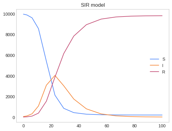
Before fitting, we need data. Let’s generate synthetic data from an SIR model with known parameters, then add realistic noise.

# True parameters
TRUE_BETA = 0.4
TRUE_GAMMA = 0.1
TOTAL_POPULATION = 10000
INITIAL_INFECTED = 50

# Generate ground truth data
ground_truth_model = SIR()
ground_truth_model(
    inits=[TOTAL_POPULATION - INITIAL_INFECTED, INITIAL_INFECTED, 0],
    trange=[0, 100],
    totpop=TOTAL_POPULATION,
    params={'beta': TRUE_BETA, 'gamma': TRUE_GAMMA},
)

# Extract time series
true_times = ground_truth_model.traces['time']
true_I = ground_truth_model.traces['I']
true_R = ground_truth_model.traces['R']

print(f"Ground truth parameters: beta={TRUE_BETA}, gamma={TRUE_GAMMA}")
print(f"R0 = {TRUE_BETA / TRUE_GAMMA:.1f}")
print(f"Time points: {len(true_times)}")

Ground truth parameters: beta=0.4, gamma=0.1
R0 = 4.0
Time points: 19

ground_truth_model.plot_traces()

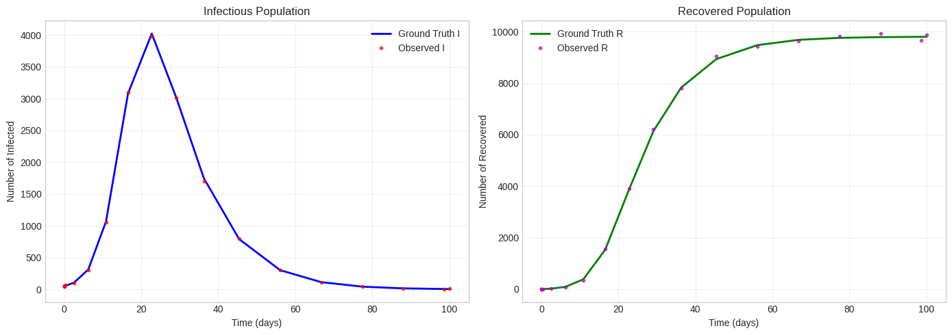
# Add realistic noise to simulate observations
# Using Poisson noise (appropriate for count data)
observed_I = np.random.poisson(lam=true_I).astype(float)
observed_R = np.random.poisson(lam=true_R).astype(float)

# Ensure non-negative
observed_I = np.maximum(observed_I, 0)
observed_R = np.maximum(observed_R, 0)

# Plot ground truth vs observed
fig, axes = plt.subplots(1, 2, figsize=(14, 5))

axes[0].plot(true_times, true_I, 'b-', label='Ground Truth I', linewidth=2)
axes[0].plot(true_times, observed_I, 'ro', label='Observed I', markersize=3, alpha=0.7)
axes[0].set_xlabel('Time (days)')
axes[0].set_ylabel('Number of Infected')
axes[0].set_title('Infectious Population')
axes[0].legend()

axes[1].plot(true_times, true_R, 'g-', label='Ground Truth R', linewidth=2)
axes[1].plot(true_times, observed_R, 'mo', label='Observed R', markersize=3, alpha=0.7)
axes[1].set_xlabel('Time (days)')
axes[1].set_ylabel('Number of Recovered')
axes[1].set_title('Recovered Population')
axes[1].legend()

plt.tight_layout()
plt.show()

3. Basic Fitting Workflow

The basic workflow consists of:

1. Create a Dataset and register observed data

2. Define ParameterSpec for parameters to fit

3. Create a ModelFitter with model, data, and specifications

4. Call fit() and analyze results

3.1 Register Data with Dataset

# Create a fresh model for fitting
model = SIR()

# Create dataset and register observed data
dataset = Dataset(model)

# Register the 'I' compartment data
dataset.register(
    name='infected',
    values=observed_I,
    times=true_times,
    state_variable='I',
    time_unit='days',
)

# Validate the dataset
validation_result = dataset.validate(total_population=TOTAL_POPULATION)
print(f"Dataset valid: {validation_result.is_valid}")
print(f"Time range: {dataset.time_range}")
print(dataset)

Dataset valid: True
Time range: (0.0, 100.0)
Dataset(n_series=1, variables=['I'], time_range=(0.0, 100.0))

3.2 Define Parameters to Fit

# Define parameter specifications
param_specs = [
    ParameterSpec(
        name='beta',
        bounds=(0.1, 1.0),
        initial=0.5,  # Initial guess
    ),
    ParameterSpec(
        name='gamma',
        bounds=(0.01, 0.5),
        initial=0.2,  # Initial guess
    ),
]

print("Parameters to fit:")
for spec in param_specs:
    print(f"  {spec.name}: bounds={spec.bounds}, initial={spec.initial}")

Parameters to fit:
  beta: bounds=(0.1, 1.0), initial=0.5
  gamma: bounds=(0.01, 0.5), initial=0.2

3.3 Create Fitter and Fit

# Create the fitter
fitter = ModelFitter(
    model=model,
    dataset=dataset,
    parameters_to_fit=param_specs,
    total_population=TOTAL_POPULATION,
    optimizer=ScipyOptimizer(method='L-BFGS-B', max_iterations=200),
)

# Perform the fit
result = fitter.fit()

# Display results
print("\n" + "="*50)
print("FITTING RESULTS")
print("="*50)
print(f"Convergence: {result.convergence}")
print(f"Number of evaluations: {result.n_evaluations}")
print(f"Final loss: {result.best_loss:.2f}")
print("\nFitted parameters:")
for param, value in result.best_params.items():
    true_val = TRUE_BETA if param == 'beta' else TRUE_GAMMA
    error = abs(value - true_val) / true_val * 100
    print(f"  {param}: {value:.4f} (true: {true_val}, error: {error:.1f}%)")

==================================================
FITTING RESULTS
==================================================
Convergence: True
Number of evaluations: 60
Final loss: 2860.33

Fitted parameters:
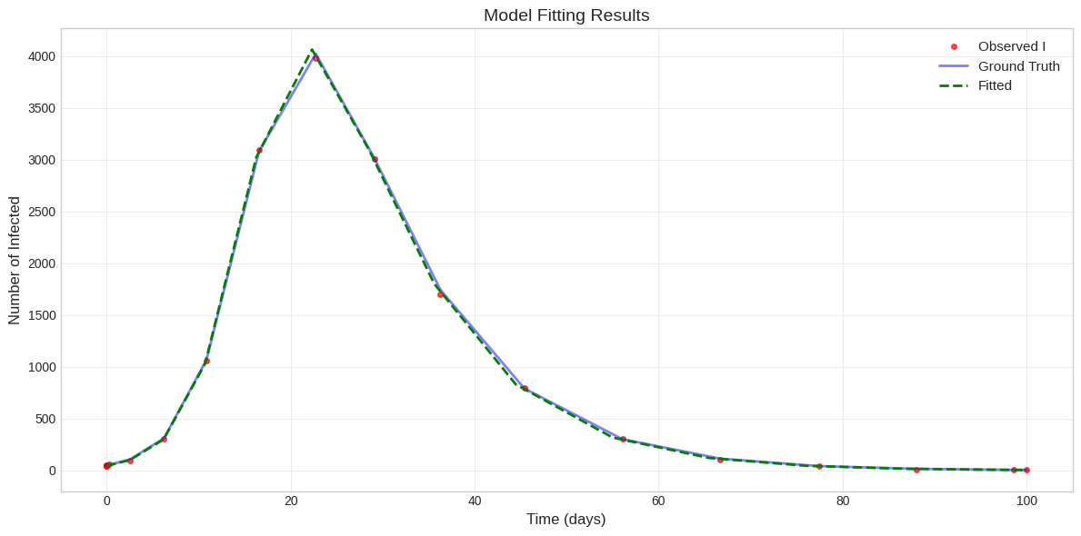
  beta: 0.4067 (true: 0.4, error: 1.7%)
  gamma: 0.1008 (true: 0.1, error: 0.8%)

3.4 Visualize Fit Results

# Plot observed vs fitted
fitted_model = result.fitted_model

fig, ax = plt.subplots(figsize=(12, 6))

# Observed data
ax.plot(true_times, observed_I, 'ro', label='Observed I', markersize=4, alpha=0.7)

# Ground truth
ax.plot(true_times, true_I, 'b-', label='Ground Truth', linewidth=2, alpha=0.5)

# Fitted model
if fitted_model is not None and fitted_model.traces:
    ax.plot(fitted_model.traces['time'], fitted_model.traces['I'],
            'g--', label='Fitted', linewidth=2)

ax.set_xlabel('Time (days)', fontsize=12)
ax.set_ylabel('Number of Infected', fontsize=12)
ax.set_title('Model Fitting Results', fontsize=14)
ax.legend(fontsize=11)
plt.tight_layout()
plt.show()

4. Data Registration and Validation

The Dataset class provides robust data handling with validation.

4.1 Registering Multiple Data Series

# Register both I and R compartments
model2 = SIR()
dataset2 = Dataset(model2)

dataset2.register(
    name='infected',
    values=observed_I,
    times=true_times,
    state_variable='I',
).register(
    name='recovered',
    values=observed_R,
    times=true_times,
    state_variable='R',
)

print(f"Registered series: {list(dataset2.series.keys())}")
print(f"State variables mapped: {list(set(s.state_variable for s in dataset2.series.values()))}")

Registered series: ['infected', 'recovered']
State variables mapped: ['I', 'R']

4.2 Validation Errors

# Example: Invalid state variable
from epimodels.fitting import DataValidationError

model_test = SIR()
dataset_test = Dataset(model_test)

dataset_test.register(
    name='invalid',
    values=observed_I,
    times=true_times,
    state_variable='X',  # 'X' doesn't exist in SIR model
)

validation = dataset_test.validate()
print(f"Valid: {validation.is_valid}")
print(f"Errors: {validation.errors}")

Valid: False
Errors: ["Series 'invalid': state variable 'X' not found in model. Available: ['I', 'S', 'R']", "Data mapped to non-existent variables: ['X']"]

4.3 Time Unit Handling

# Data with different time units
model3 = SIR()
dataset3 = Dataset(model3)

# Register with weeks instead of days
weeks = true_times / 7.0

dataset3.register(
    name='infected_weekly',
    values=observed_I,
    times=weeks,
    state_variable='I',
    time_unit='weeks',
)

print(f"Dataset time unit: {dataset3.time_unit}")
print(f"Series time unit: {dataset3.series['infected_weekly'].time_unit}")
print(f"Time range: {dataset3.time_range}")

Dataset time unit: weeks
Series time unit: weeks
Time range: (0.0, 14.285714285714286)

4.4 DataFrame Integration

import pandas as pd

# Create a DataFrame with observations
df = pd.DataFrame({
    'day': true_times,
    'cases': observed_I,
    'recoveries': observed_R,
})

print("Sample data:")
display(df.head(10))

# Register from DataFrame
model_df = SIR()
dataset_df = Dataset(model_df)

dataset_df.register_from_dataframe(
    df=df,
    time_column='day',
    mapping={'cases': 'I', 'recoveries': 'R'},
    time_unit='days',
)

print(f"\nRegistered from DataFrame: {list(dataset_df.series.keys())}")

Sample data:

	day	cases	recoveries
0	0.000000	47.0	0.0
1	0.000283	55.0	0.0
2	0.003111	42.0	0.0
3	0.031395	53.0	0.0
4	0.314235	63.0	1.0
5	2.552370	96.0	24.0
6	6.256865	302.0	84.0
7	10.862630	1062.0	354.0
8	16.573157	3099.0	1564.0
9	22.737625	3986.0	3898.0

Registered from DataFrame: ['cases', 'recoveries']

5. Loss Functions

Different loss functions are appropriate for different data types and noise models.

5.1 Available Loss Functions

loss_functions = {
    'SSE': SumOfSquaredErrors(),
    'Poisson': PoissonLikelihood(),
    'NegBinom': NegativeBinomialLikelihood(dispersion=5.0),
    'Normal': NormalLikelihood(),
    'Huber': HuberLoss(delta=10.0),
}

print("Available loss functions:")
for name, lf in loss_functions.items():
    print(f"  - {name}: {lf.__class__.__name__}")

Available loss functions:
  - SSE: SumOfSquaredErrors
  - Poisson: PoissonLikelihood
  - NegBinom: NegativeBinomialLikelihood
  - Normal: NormalLikelihood
  - Huber: HuberLoss

5.2 Comparing Loss Functions

# Fit with different loss functions
results_comparison = {}

for name, loss_fn in loss_functions.items():
    print(f"Fitting with {name}...")

    fitter_comp = ModelFitter(
        model=SIR(),
        dataset=dataset,  # Using single-series dataset from earlier
        parameters_to_fit=param_specs,
        total_population=TOTAL_POPULATION,
        loss_fn=loss_fn,
        optimizer=ScipyOptimizer(method='L-BFGS-B', max_iterations=100),
    )

    result = fitter_comp.fit()
    results_comparison[name] = result

Fitting with SSE...
Fitting with Poisson...
Fitting with NegBinom...
Fitting with Normal...
Fitting with Huber...

# Compare results
print("\n" + "="*70)
print("LOSS FUNCTION COMPARISON")
print("="*70)
print(f"{'Loss Function':<15} {'beta':>10} {'gamma':>10} {'R0':>10} {'Loss':>12}")
print("-"*70)
print(f"{'TRUE VALUES':<15} {TRUE_BETA:>10.4f} {TRUE_GAMMA:>10.4f} {TRUE_BETA/TRUE_GAMMA:>10.2f} {'-':>12}")
print("-"*70)

for name, result in results_comparison.items():
    beta = result.best_params['beta']
    gamma = result.best_params['gamma']
    r0 = beta / gamma
    print(f"{name:<15} {beta:>10.4f} {gamma:>10.4f} {r0:>10.2f} {result.best_loss:>12.2f}")

======================================================================
LOSS FUNCTION COMPARISON
======================================================================
Loss Function         beta      gamma         R0         Loss
----------------------------------------------------------------------
TRUE VALUES         0.4000     0.1000       4.00            -
----------------------------------------------------------------------
SSE                 0.4067     0.1008       4.03      2860.33
Poisson             0.4057     0.1008       4.03       143.37
NegBinom            0.3994     0.1007       3.97       201.01
Normal              0.4067     0.1008       4.03        74.61
Huber               0.4056     0.1007       4.03      1068.47

5.3 When to Use Each Loss Function

Loss Function	Best For	Assumptions
SSE	General purpose	Gaussian errors
Poisson	Count data	Mean = Variance
Negative Binomial	Overdispersed counts	Variance > Mean
Normal	Continuous measurements	Known or estimated σ
Huber	Data with outliers	Robust to outliers

6. Optimizers

The module supports multiple optimization backends.

6.1 Scipy Methods

# Compare scipy optimization methods
scipy_methods = ['L-BFGS-B', 'Nelder-Mead', 'Powell', 'differential_evolution']
optimizer_results = {}

for method in scipy_methods:
    print(f"Testing {method}...")

    optimizer = ScipyOptimizer(method=method, max_iterations=100)

    fitter_opt = ModelFitter(
        model=SIR(),
        dataset=dataset,
        parameters_to_fit=param_specs,
        total_population=TOTAL_POPULATION,
        optimizer=optimizer,
    )

    result = fitter_opt.fit()
    optimizer_results[method] = result

Testing L-BFGS-B...
Testing Nelder-Mead...
Testing Powell...
Testing differential_evolution...

# Compare optimizer performance
print("\n" + "="*80)
print("OPTIMIZER COMPARISON")
print("="*80)
print(f"{'Method':<25} {'beta':>10} {'gamma':>10} {'Evals':>8} {'Converged':>10}")
print("-"*80)

for method, result in optimizer_results.items():
    beta = result.best_params['beta']
    gamma = result.best_params['gamma']
    print(f"{method:<25} {beta:>10.4f} {gamma:>10.4f} {result.n_evaluations:>8} {str(result.convergence):>10}")

================================================================================
OPTIMIZER COMPARISON
================================================================================
Method                          beta      gamma    Evals  Converged
--------------------------------------------------------------------------------
L-BFGS-B                      0.4067     0.1008       60       True
Nelder-Mead                   0.4067     0.1008       60       True
Powell                        0.4067     0.1008       60       True
differential_evolution        0.4067     0.1008     1164       True

6.2 Multi-Start Optimization

For robust results, especially with local minima, use multi-start optimization.

# Multi-start optimization
base_optimizer = ScipyOptimizer(method='L-BFGS-B', max_iterations=50)
multi_start = MultiStartOptimizer(
    base_optimizer=base_optimizer,
    n_starts=5,
    sampling_method='latin_hypercube',
    seed=42,
)

fitter_ms = ModelFitter(
    model=SIR(),
    dataset=dataset,
    parameters_to_fit=param_specs,
    total_population=TOTAL_POPULATION,
    optimizer=multi_start,
)

result_ms = fitter_ms.fit()

print(f"Multi-start optimization results:")
print(f"  beta: {result_ms.best_params['beta']:.4f}")
print(f"  gamma: {result_ms.best_params['gamma']:.4f}")
print(f"  Total evaluations: {result_ms.n_evaluations}")

Multi-start optimization results:
  beta: 0.4067
  gamma: 0.1008
  Total evaluations: 477

7. Advanced Features

7.1 Fixed Parameters

Sometimes we know some parameters and only want to fit others.

# Fix gamma and only fit beta
fitter_fixed = ModelFitter(
    model=SIR(),
    dataset=dataset,
    parameters_to_fit=[
        ParameterSpec(name='beta', bounds=(0.1, 1.0), initial=0.5),
    ],
    total_population=TOTAL_POPULATION,
    fixed_params={'gamma': TRUE_GAMMA},  # Fix gamma at true value
)

result_fixed = fitter_fixed.fit()

print("Fitting with fixed gamma:")
print(f"  Fitted beta: {result_fixed.best_params['beta']:.4f} (true: {TRUE_BETA})")
print(f"  Fixed gamma: {TRUE_GAMMA}")

Fitting with fixed gamma:
  Fitted beta: 0.4064 (true: 0.4)
  Fixed gamma: 0.1

7.2 Log-Scale Parameter Transformation

For parameters spanning orders of magnitude, log-scale transformation can improve optimization.

# =noisy_I,# Parameters with log-scale transformation
param_specs_log = [
    ParameterSpec(
        name='beta',
        bounds=(0.01, 1.0),
        initial=0.3,
        log_scale=True,  # Search in log space
    ),
    ParameterSpec(
        name='gamma',
        bounds=(0.01, 0.5),
        initial=0.1,
        log_scale=True,  # Search in log space
    ),
]

print("Log-scale parameter specs:")
for spec in param_specs_log:
    print(f"  {spec.name}: bounds={spec.bounds}, log_scale={spec.log_scale}")

Log-scale parameter specs:
  beta: bounds=(0.01, 1.0), log_scale=True
  gamma: bounds=(0.01, 0.5), log_scale=True

7.3 Profile Likelihood for Confidence Intervals

# Compute profile likelihood for beta
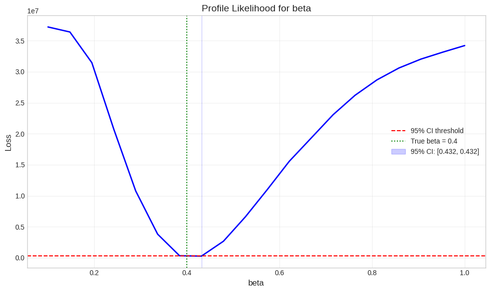
profile_result = fitter.profile_likelihood(
    param_name='beta',
    n_points=20,
    threshold=3.84,  # Chi-squared 95% CI for 1 df
)

print("Profile likelihood analysis for beta:")
print(f"  Minimum loss: {profile_result['min_loss']:.2f}")
print(f"  95% CI threshold: {profile_result['threshold_loss']:.2f}")
print(f"  Confidence interval: {profile_result['confidence_interval']}")

Profile likelihood analysis for beta:
  Minimum loss: 283984.09
  95% CI threshold: 283986.01
  Confidence interval: (np.float64(0.43157894736842106), np.float64(0.43157894736842106))

# Plot profile likelihood
fig, ax = plt.subplots(figsize=(10, 6))

ax.plot(profile_result['values'], profile_result['losses'], 'b-', linewidth=2)
ax.axhline(y=profile_result['threshold_loss'], color='r', linestyle='--',
           label=f"95% CI threshold")
ax.axvline(x=TRUE_BETA, color='g', linestyle=':', label=f"True beta = {TRUE_BETA}")

# Shade CI region
ci = profile_result['confidence_interval']
if ci[0] is not None and ci[1] is not None:
    ax.axvspan(ci[0], ci[1], alpha=0.2, color='blue', label=f"95% CI: [{ci[0]:.3f}, {ci[1]:.3f}]")

ax.set_xlabel('beta', fontsize=12)
ax.set_ylabel('Loss', fontsize=12)
ax.set_title('Profile Likelihood for beta', fontsize=14)
ax.legend(fontsize=10)
plt.tight_layout()
plt.show()

7.4 Fitting Initial Conditions

By default, initial conditions are estimated from the first data point and kept fixed. You can also fit initial conditions alongside model parameters using fit_initial_conditions=True.

For more control, use InitialConditionSpec to specify:

• bounds: Search range for the initial value

• initial: Starting value for optimization

• fixed: If True, the IC is held fixed during fitting

This allows you to fix some initial conditions (e.g., S[0] = N - I[0] - R[0]) while fitting others.

# Example: Fit initial conditions for I and R, but fix S based on total population
from epimodels.fitting import InitialConditionSpec

# Create dataset with both I and R observations
model_ic = SIR()
dataset_ic = Dataset(model_ic)
dataset_ic.register(
    name='infected',
    values=observed_I,
    times=true_times,
    state_variable='I',
).register(
    name='recovered',
    values=observed_R,
    times=true_times,
    state_variable='R',
)

# Specify IC fitting: fix S[0], fit I[0] and R[0]
# S[0] will be computed as: TOTAL_POPULATION - I[0] - R[0]
ic_specs = [
    InitialConditionSpec(
        state_variable='S',
        bounds=(TOTAL_POPULATION - 100, TOTAL_POPULATION),
        initial=TOTAL_POPULATION - INITIAL_INFECTED,
        fixed=False,  # Fixed - will be computed from other ICs
    ),
    InitialConditionSpec(
        state_variable='I',
        bounds=(1, 500),
        initial=INITIAL_INFECTED,
        fixed=True,  # Will be fitted
    ),
    InitialConditionSpec(
        state_variable='R',
        bounds=(0, 100),
        initial=0,
        fixed=False,  # Will be fitted
    ),
]

# Create fitter with IC fitting enabled
fitter_ic = ModelFitter(
    model=model_ic,
    dataset=dataset_ic,
    parameters_to_fit=[
        ParameterSpec(name='beta', bounds=(0.1, 1.0), initial=0.5),
        ParameterSpec(name='gamma', bounds=(0.01, 0.5), initial=0.2),
    ],
    total_population=TOTAL_POPULATION,
    fit_initial_conditions=True,
    initial_condition_specs=ic_specs,
)

# Fit the model
result_ic = fitter_ic.fit()

print("Fitting with initial conditions:")
print(f"  Fitted beta: {result_ic.best_params['beta']:.4f} (true: {TRUE_BETA})")
print(f"  Fitted gamma: {result_ic.best_params['gamma']:.4f} (true: {TRUE_GAMMA})")
print(f"  Fitted I[0]: {result_ic.best_initial_conditions[1]:.1f} (true: {INITIAL_INFECTED})")
print(f"  Fitted R[0]: {result_ic.best_initial_conditions[2]:.1f} (true: 0)")
print(f"  Fixed S[0]: {result_ic.best_initial_conditions[0]:.1f}")

/home/fccoelho/Documentos/Software_projects/epimodels/epimodels/fitting/base.py:412: RuntimeWarning: Model evaluation failed: Sum of initial conditions (10150.0) exceeds total population (10000)
  warnings.warn(f"Model evaluation failed: {e}", RuntimeWarning)
/home/fccoelho/Documentos/Software_projects/epimodels/epimodels/fitting/base.py:412: RuntimeWarning: Model evaluation failed: Sum of initial conditions (10149.99999999) exceeds total population (10000)
  warnings.warn(f"Model evaluation failed: {e}", RuntimeWarning)
/home/fccoelho/Documentos/Software_projects/epimodels/epimodels/fitting/base.py:412: RuntimeWarning: Model evaluation failed: Sum of initial conditions (10037.678751579851) exceeds total population (10000)
  warnings.warn(f"Model evaluation failed: {e}", RuntimeWarning)
/home/fccoelho/Documentos/Software_projects/epimodels/epimodels/fitting/base.py:412: RuntimeWarning: Model evaluation failed: Sum of initial conditions (10037.678751589852) exceeds total population (10000)
  warnings.warn(f"Model evaluation failed: {e}", RuntimeWarning)
/home/fccoelho/Documentos/Software_projects/epimodels/epimodels/fitting/base.py:412: RuntimeWarning: Model evaluation failed: Sum of initial conditions (10011.246044332569) exceeds total population (10000)
  warnings.warn(f"Model evaluation failed: {e}", RuntimeWarning)
/home/fccoelho/Documentos/Software_projects/epimodels/epimodels/fitting/base.py:412: RuntimeWarning: Model evaluation failed: Sum of initial conditions (10011.24604434257) exceeds total population (10000)
  warnings.warn(f"Model evaluation failed: {e}", RuntimeWarning)
/home/fccoelho/Documentos/Software_projects/epimodels/epimodels/fitting/base.py:412: RuntimeWarning: Model evaluation failed: Sum of initial conditions (10011.246044342568) exceeds total population (10000)
  warnings.warn(f"Model evaluation failed: {e}", RuntimeWarning)
/home/fccoelho/Documentos/Software_projects/epimodels/epimodels/fitting/base.py:412: RuntimeWarning: Model evaluation failed: Sum of initial conditions (10010.25094652309) exceeds total population (10000)
  warnings.warn(f"Model evaluation failed: {e}", RuntimeWarning)
/home/fccoelho/Documentos/Software_projects/epimodels/epimodels/fitting/base.py:412: RuntimeWarning: Model evaluation failed: Sum of initial conditions (10010.250946533091) exceeds total population (10000)
  warnings.warn(f"Model evaluation failed: {e}", RuntimeWarning)
/home/fccoelho/Documentos/Software_projects/epimodels/epimodels/fitting/base.py:412: RuntimeWarning: Model evaluation failed: Sum of initial conditions (10010.25094653309) exceeds total population (10000)
  warnings.warn(f"Model evaluation failed: {e}", RuntimeWarning)
/home/fccoelho/Documentos/Software_projects/epimodels/epimodels/fitting/base.py:412: RuntimeWarning: Model evaluation failed: Sum of initial conditions (10010.002172119051) exceeds total population (10000)
  warnings.warn(f"Model evaluation failed: {e}", RuntimeWarning)
/home/fccoelho/Documentos/Software_projects/epimodels/epimodels/fitting/base.py:412: RuntimeWarning: Model evaluation failed: Sum of initial conditions (10010.002172129052) exceeds total population (10000)
  warnings.warn(f"Model evaluation failed: {e}", RuntimeWarning)
/home/fccoelho/Documentos/Software_projects/epimodels/epimodels/fitting/base.py:412: RuntimeWarning: Model evaluation failed: Sum of initial conditions (10149.962619408532) exceeds total population (10000)
  warnings.warn(f"Model evaluation failed: {e}", RuntimeWarning)
/home/fccoelho/Documentos/Software_projects/epimodels/epimodels/fitting/base.py:412: RuntimeWarning: Model evaluation failed: Sum of initial conditions (10149.962619398531) exceeds total population (10000)
  warnings.warn(f"Model evaluation failed: {e}", RuntimeWarning)
/home/fccoelho/Documentos/Software_projects/epimodels/epimodels/fitting/base.py:412: RuntimeWarning: Model evaluation failed: Sum of initial conditions (10149.962619418533) exceeds total population (10000)
  warnings.warn(f"Model evaluation failed: {e}", RuntimeWarning)
/home/fccoelho/Documentos/Software_projects/epimodels/epimodels/fitting/base.py:412: RuntimeWarning: Model evaluation failed: Sum of initial conditions (10079.858433258289) exceeds total population (10000)
  warnings.warn(f"Model evaluation failed: {e}", RuntimeWarning)
/home/fccoelho/Documentos/Software_projects/epimodels/epimodels/fitting/base.py:412: RuntimeWarning: Model evaluation failed: Sum of initial conditions (10079.85843326829) exceeds total population (10000)
  warnings.warn(f"Model evaluation failed: {e}", RuntimeWarning)
/home/fccoelho/Documentos/Software_projects/epimodels/epimodels/fitting/base.py:412: RuntimeWarning: Model evaluation failed: Sum of initial conditions (10079.858433268288) exceeds total population (10000)
  warnings.warn(f"Model evaluation failed: {e}", RuntimeWarning)
/home/fccoelho/Documentos/Software_projects/epimodels/epimodels/fitting/base.py:412: RuntimeWarning: Model evaluation failed: Sum of initial conditions (10044.806554293556) exceeds total population (10000)
  warnings.warn(f"Model evaluation failed: {e}", RuntimeWarning)
/home/fccoelho/Documentos/Software_projects/epimodels/epimodels/fitting/base.py:412: RuntimeWarning: Model evaluation failed: Sum of initial conditions (10044.806554303557) exceeds total population (10000)
  warnings.warn(f"Model evaluation failed: {e}", RuntimeWarning)
/home/fccoelho/Documentos/Software_projects/epimodels/epimodels/fitting/base.py:412: RuntimeWarning: Model evaluation failed: Sum of initial conditions (10027.280668121946) exceeds total population (10000)
  warnings.warn(f"Model evaluation failed: {e}", RuntimeWarning)
/home/fccoelho/Documentos/Software_projects/epimodels/epimodels/fitting/base.py:412: RuntimeWarning: Model evaluation failed: Sum of initial conditions (10027.280668131947) exceeds total population (10000)
  warnings.warn(f"Model evaluation failed: {e}", RuntimeWarning)
/home/fccoelho/Documentos/Software_projects/epimodels/epimodels/fitting/base.py:412: RuntimeWarning: Model evaluation failed: Sum of initial conditions (10018.517738323637) exceeds total population (10000)
  warnings.warn(f"Model evaluation failed: {e}", RuntimeWarning)
/home/fccoelho/Documentos/Software_projects/epimodels/epimodels/fitting/base.py:412: RuntimeWarning: Model evaluation failed: Sum of initial conditions (10018.517738333638) exceeds total population (10000)
  warnings.warn(f"Model evaluation failed: {e}", RuntimeWarning)
/home/fccoelho/Documentos/Software_projects/epimodels/epimodels/fitting/base.py:412: RuntimeWarning: Model evaluation failed: Sum of initial conditions (10014.13699951408) exceeds total population (10000)
  warnings.warn(f"Model evaluation failed: {e}", RuntimeWarning)
/home/fccoelho/Documentos/Software_projects/epimodels/epimodels/fitting/base.py:412: RuntimeWarning: Model evaluation failed: Sum of initial conditions (10014.13699952408) exceeds total population (10000)
  warnings.warn(f"Model evaluation failed: {e}", RuntimeWarning)
/home/fccoelho/Documentos/Software_projects/epimodels/epimodels/fitting/base.py:412: RuntimeWarning: Model evaluation failed: Sum of initial conditions (10011.946748875098) exceeds total population (10000)
  warnings.warn(f"Model evaluation failed: {e}", RuntimeWarning)
/home/fccoelho/Documentos/Software_projects/epimodels/epimodels/fitting/base.py:412: RuntimeWarning: Model evaluation failed: Sum of initial conditions (10011.946748885099) exceeds total population (10000)
  warnings.warn(f"Model evaluation failed: {e}", RuntimeWarning)
/home/fccoelho/Documentos/Software_projects/epimodels/epimodels/fitting/base.py:412: RuntimeWarning: Model evaluation failed: Sum of initial conditions (10011.946748885097) exceeds total population (10000)
  warnings.warn(f"Model evaluation failed: {e}", RuntimeWarning)
/home/fccoelho/Documentos/Software_projects/epimodels/epimodels/fitting/base.py:412: RuntimeWarning: Model evaluation failed: Sum of initial conditions (10141.878067286249) exceeds total population (10000)
  warnings.warn(f"Model evaluation failed: {e}", RuntimeWarning)
/home/fccoelho/Documentos/Software_projects/epimodels/epimodels/fitting/base.py:412: RuntimeWarning: Model evaluation failed: Sum of initial conditions (10141.87806729625) exceeds total population (10000)
  warnings.warn(f"Model evaluation failed: {e}", RuntimeWarning)
/home/fccoelho/Documentos/Software_projects/epimodels/epimodels/fitting/base.py:412: RuntimeWarning: Model evaluation failed: Sum of initial conditions (10141.878067276248) exceeds total population (10000)
  warnings.warn(f"Model evaluation failed: {e}", RuntimeWarning)
/home/fccoelho/Documentos/Software_projects/epimodels/epimodels/fitting/base.py:412: RuntimeWarning: Model evaluation failed: Sum of initial conditions (10075.8206951335) exceeds total population (10000)
  warnings.warn(f"Model evaluation failed: {e}", RuntimeWarning)
/home/fccoelho/Documentos/Software_projects/epimodels/epimodels/fitting/base.py:412: RuntimeWarning: Model evaluation failed: Sum of initial conditions (10075.8206951435) exceeds total population (10000)
  warnings.warn(f"Model evaluation failed: {e}", RuntimeWarning)
/home/fccoelho/Documentos/Software_projects/epimodels/epimodels/fitting/base.py:412: RuntimeWarning: Model evaluation failed: Sum of initial conditions (10075.820695143499) exceeds total population (10000)
  warnings.warn(f"Model evaluation failed: {e}", RuntimeWarning)
/home/fccoelho/Documentos/Software_projects/epimodels/epimodels/fitting/base.py:412: RuntimeWarning: Model evaluation failed: Sum of initial conditions (10010.094218228329) exceeds total population (10000)
  warnings.warn(f"Model evaluation failed: {e}", RuntimeWarning)
/home/fccoelho/Documentos/Software_projects/epimodels/epimodels/fitting/base.py:412: RuntimeWarning: Model evaluation failed: Sum of initial conditions (10010.09421823833) exceeds total population (10000)
  warnings.warn(f"Model evaluation failed: {e}", RuntimeWarning)
/home/fccoelho/Documentos/Software_projects/epimodels/epimodels/fitting/base.py:412: RuntimeWarning: Model evaluation failed: Sum of initial conditions (10010.04010036447) exceeds total population (10000)
  warnings.warn(f"Model evaluation failed: {e}", RuntimeWarning)
/home/fccoelho/Documentos/Software_projects/epimodels/epimodels/fitting/base.py:412: RuntimeWarning: Model evaluation failed: Sum of initial conditions (10010.04010037447) exceeds total population (10000)
  warnings.warn(f"Model evaluation failed: {e}", RuntimeWarning)
/home/fccoelho/Documentos/Software_projects/epimodels/epimodels/fitting/base.py:412: RuntimeWarning: Model evaluation failed: Sum of initial conditions (10010.013041433149) exceeds total population (10000)
  warnings.warn(f"Model evaluation failed: {e}", RuntimeWarning)
/home/fccoelho/Documentos/Software_projects/epimodels/epimodels/fitting/base.py:412: RuntimeWarning: Model evaluation failed: Sum of initial conditions (10010.01304144315) exceeds total population (10000)
  warnings.warn(f"Model evaluation failed: {e}", RuntimeWarning)
/home/fccoelho/Documentos/Software_projects/epimodels/epimodels/fitting/base.py:412: RuntimeWarning: Model evaluation failed: Sum of initial conditions (10010.008441414833) exceeds total population (10000)
  warnings.warn(f"Model evaluation failed: {e}", RuntimeWarning)
/home/fccoelho/Documentos/Software_projects/epimodels/epimodels/fitting/base.py:412: RuntimeWarning: Model evaluation failed: Sum of initial conditions (10010.008441424834) exceeds total population (10000)
  warnings.warn(f"Model evaluation failed: {e}", RuntimeWarning)
/home/fccoelho/Documentos/Software_projects/epimodels/epimodels/fitting/base.py:412: RuntimeWarning: Model evaluation failed: Sum of initial conditions (10010.857593866049) exceeds total population (10000)
  warnings.warn(f"Model evaluation failed: {e}", RuntimeWarning)
/home/fccoelho/Documentos/Software_projects/epimodels/epimodels/fitting/base.py:412: RuntimeWarning: Model evaluation failed: Sum of initial conditions (10010.85759387605) exceeds total population (10000)
  warnings.warn(f"Model evaluation failed: {e}", RuntimeWarning)
/home/fccoelho/Documentos/Software_projects/epimodels/epimodels/fitting/base.py:412: RuntimeWarning: Model evaluation failed: Sum of initial conditions (10010.857593876048) exceeds total population (10000)
  warnings.warn(f"Model evaluation failed: {e}", RuntimeWarning)
/home/fccoelho/Documentos/Software_projects/epimodels/epimodels/fitting/base.py:412: RuntimeWarning: Model evaluation failed: Sum of initial conditions (10010.428552967584) exceeds total population (10000)
  warnings.warn(f"Model evaluation failed: {e}", RuntimeWarning)
/home/fccoelho/Documentos/Software_projects/epimodels/epimodels/fitting/base.py:412: RuntimeWarning: Model evaluation failed: Sum of initial conditions (10010.428552977584) exceeds total population (10000)
  warnings.warn(f"Model evaluation failed: {e}", RuntimeWarning)
/home/fccoelho/Documentos/Software_projects/epimodels/epimodels/fitting/base.py:412: RuntimeWarning: Model evaluation failed: Sum of initial conditions (10010.214032547216) exceeds total population (10000)
  warnings.warn(f"Model evaluation failed: {e}", RuntimeWarning)
/home/fccoelho/Documentos/Software_projects/epimodels/epimodels/fitting/base.py:412: RuntimeWarning: Model evaluation failed: Sum of initial conditions (10010.214032557216) exceeds total population (10000)
  warnings.warn(f"Model evaluation failed: {e}", RuntimeWarning)
/home/fccoelho/Documentos/Software_projects/epimodels/epimodels/fitting/base.py:412: RuntimeWarning: Model evaluation failed: Sum of initial conditions (10010.106772344796) exceeds total population (10000)
  warnings.warn(f"Model evaluation failed: {e}", RuntimeWarning)
/home/fccoelho/Documentos/Software_projects/epimodels/epimodels/fitting/base.py:412: RuntimeWarning: Model evaluation failed: Sum of initial conditions (10010.106772354797) exceeds total population (10000)
  warnings.warn(f"Model evaluation failed: {e}", RuntimeWarning)
/home/fccoelho/Documentos/Software_projects/epimodels/epimodels/fitting/base.py:412: RuntimeWarning: Model evaluation failed: Sum of initial conditions (10010.053142358962) exceeds total population (10000)
  warnings.warn(f"Model evaluation failed: {e}", RuntimeWarning)
/home/fccoelho/Documentos/Software_projects/epimodels/epimodels/fitting/base.py:412: RuntimeWarning: Model evaluation failed: Sum of initial conditions (10010.053142368963) exceeds total population (10000)
  warnings.warn(f"Model evaluation failed: {e}", RuntimeWarning)
/home/fccoelho/Documentos/Software_projects/epimodels/epimodels/fitting/base.py:412: RuntimeWarning: Model evaluation failed: Sum of initial conditions (10010.026327366257) exceeds total population (10000)
  warnings.warn(f"Model evaluation failed: {e}", RuntimeWarning)
/home/fccoelho/Documentos/Software_projects/epimodels/epimodels/fitting/base.py:412: RuntimeWarning: Model evaluation failed: Sum of initial conditions (10010.026327376258) exceeds total population (10000)
  warnings.warn(f"Model evaluation failed: {e}", RuntimeWarning)
/home/fccoelho/Documentos/Software_projects/epimodels/epimodels/fitting/base.py:412: RuntimeWarning: Model evaluation failed: Sum of initial conditions (10010.026327376256) exceeds total population (10000)
  warnings.warn(f"Model evaluation failed: {e}", RuntimeWarning)
/home/fccoelho/Documentos/Software_projects/epimodels/epimodels/fitting/base.py:412: RuntimeWarning: Model evaluation failed: Sum of initial conditions (10010.85884101824) exceeds total population (10000)
  warnings.warn(f"Model evaluation failed: {e}", RuntimeWarning)
/home/fccoelho/Documentos/Software_projects/epimodels/epimodels/fitting/base.py:412: RuntimeWarning: Model evaluation failed: Sum of initial conditions (10010.858841028241) exceeds total population (10000)
  warnings.warn(f"Model evaluation failed: {e}", RuntimeWarning)
/home/fccoelho/Documentos/Software_projects/epimodels/epimodels/fitting/base.py:412: RuntimeWarning: Model evaluation failed: Sum of initial conditions (10010.429176746948) exceeds total population (10000)
  warnings.warn(f"Model evaluation failed: {e}", RuntimeWarning)
/home/fccoelho/Documentos/Software_projects/epimodels/epimodels/fitting/base.py:412: RuntimeWarning: Model evaluation failed: Sum of initial conditions (10010.429176756948) exceeds total population (10000)
  warnings.warn(f"Model evaluation failed: {e}", RuntimeWarning)
/home/fccoelho/Documentos/Software_projects/epimodels/epimodels/fitting/base.py:412: RuntimeWarning: Model evaluation failed: Sum of initial conditions (10010.214344624053) exceeds total population (10000)
  warnings.warn(f"Model evaluation failed: {e}", RuntimeWarning)
/home/fccoelho/Documentos/Software_projects/epimodels/epimodels/fitting/base.py:412: RuntimeWarning: Model evaluation failed: Sum of initial conditions (10010.214344634054) exceeds total population (10000)
  warnings.warn(f"Model evaluation failed: {e}", RuntimeWarning)
/home/fccoelho/Documentos/Software_projects/epimodels/epimodels/fitting/base.py:412: RuntimeWarning: Model evaluation failed: Sum of initial conditions (10010.106928565787) exceeds total population (10000)
  warnings.warn(f"Model evaluation failed: {e}", RuntimeWarning)
/home/fccoelho/Documentos/Software_projects/epimodels/epimodels/fitting/base.py:412: RuntimeWarning: Model evaluation failed: Sum of initial conditions (10010.106928575788) exceeds total population (10000)
  warnings.warn(f"Model evaluation failed: {e}", RuntimeWarning)
/home/fccoelho/Documentos/Software_projects/epimodels/epimodels/fitting/base.py:412: RuntimeWarning: Model evaluation failed: Sum of initial conditions (10010.053220540518) exceeds total population (10000)
  warnings.warn(f"Model evaluation failed: {e}", RuntimeWarning)
/home/fccoelho/Documentos/Software_projects/epimodels/epimodels/fitting/base.py:412: RuntimeWarning: Model evaluation failed: Sum of initial conditions (10010.053220550519) exceeds total population (10000)
  warnings.warn(f"Model evaluation failed: {e}", RuntimeWarning)
/home/fccoelho/Documentos/Software_projects/epimodels/epimodels/fitting/base.py:412: RuntimeWarning: Model evaluation failed: Sum of initial conditions (10010.053220550517) exceeds total population (10000)
  warnings.warn(f"Model evaluation failed: {e}", RuntimeWarning)
/home/fccoelho/Documentos/Software_projects/epimodels/epimodels/fitting/base.py:412: RuntimeWarning: Model evaluation failed: Sum of initial conditions (10010.026366528082) exceeds total population (10000)
  warnings.warn(f"Model evaluation failed: {e}", RuntimeWarning)
/home/fccoelho/Documentos/Software_projects/epimodels/epimodels/fitting/base.py:412: RuntimeWarning: Model evaluation failed: Sum of initial conditions (10010.026366538083) exceeds total population (10000)
  warnings.warn(f"Model evaluation failed: {e}", RuntimeWarning)
/home/fccoelho/Documentos/Software_projects/epimodels/epimodels/fitting/base.py:412: RuntimeWarning: Model evaluation failed: Sum of initial conditions (10010.02636653808) exceeds total population (10000)
  warnings.warn(f"Model evaluation failed: {e}", RuntimeWarning)
/home/fccoelho/Documentos/Software_projects/epimodels/epimodels/fitting/base.py:412: RuntimeWarning: Model evaluation failed: Sum of initial conditions (10010.861086708797) exceeds total population (10000)
  warnings.warn(f"Model evaluation failed: {e}", RuntimeWarning)
/home/fccoelho/Documentos/Software_projects/epimodels/epimodels/fitting/base.py:412: RuntimeWarning: Model evaluation failed: Sum of initial conditions (10010.861086718798) exceeds total population (10000)
  warnings.warn(f"Model evaluation failed: {e}", RuntimeWarning)
/home/fccoelho/Documentos/Software_projects/epimodels/epimodels/fitting/base.py:412: RuntimeWarning: Model evaluation failed: Sum of initial conditions (10010.430299663643) exceeds total population (10000)
  warnings.warn(f"Model evaluation failed: {e}", RuntimeWarning)
/home/fccoelho/Documentos/Software_projects/epimodels/epimodels/fitting/base.py:412: RuntimeWarning: Model evaluation failed: Sum of initial conditions (10010.430299673644) exceeds total population (10000)
  warnings.warn(f"Model evaluation failed: {e}", RuntimeWarning)
/home/fccoelho/Documentos/Software_projects/epimodels/epimodels/fitting/base.py:412: RuntimeWarning: Model evaluation failed: Sum of initial conditions (10010.21490615387) exceeds total population (10000)
  warnings.warn(f"Model evaluation failed: {e}", RuntimeWarning)
/home/fccoelho/Documentos/Software_projects/epimodels/epimodels/fitting/base.py:412: RuntimeWarning: Model evaluation failed: Sum of initial conditions (10010.21490616387) exceeds total population (10000)
  warnings.warn(f"Model evaluation failed: {e}", RuntimeWarning)
/home/fccoelho/Documentos/Software_projects/epimodels/epimodels/fitting/base.py:412: RuntimeWarning: Model evaluation failed: Sum of initial conditions (10010.214906163868) exceeds total population (10000)
  warnings.warn(f"Model evaluation failed: {e}", RuntimeWarning)
/home/fccoelho/Documentos/Software_projects/epimodels/epimodels/fitting/base.py:412: RuntimeWarning: Model evaluation failed: Sum of initial conditions (10010.107209418502) exceeds total population (10000)
  warnings.warn(f"Model evaluation failed: {e}", RuntimeWarning)
/home/fccoelho/Documentos/Software_projects/epimodels/epimodels/fitting/base.py:412: RuntimeWarning: Model evaluation failed: Sum of initial conditions (10010.107209428503) exceeds total population (10000)
  warnings.warn(f"Model evaluation failed: {e}", RuntimeWarning)
/home/fccoelho/Documentos/Software_projects/epimodels/epimodels/fitting/base.py:412: RuntimeWarning: Model evaluation failed: Sum of initial conditions (10010.053361051625) exceeds total population (10000)
  warnings.warn(f"Model evaluation failed: {e}", RuntimeWarning)
/home/fccoelho/Documentos/Software_projects/epimodels/epimodels/fitting/base.py:412: RuntimeWarning: Model evaluation failed: Sum of initial conditions (10010.053361061626) exceeds total population (10000)
  warnings.warn(f"Model evaluation failed: {e}", RuntimeWarning)
/home/fccoelho/Documentos/Software_projects/epimodels/epimodels/fitting/base.py:412: RuntimeWarning: Model evaluation failed: Sum of initial conditions (10010.0264369209) exceeds total population (10000)
  warnings.warn(f"Model evaluation failed: {e}", RuntimeWarning)
/home/fccoelho/Documentos/Software_projects/epimodels/epimodels/fitting/base.py:412: RuntimeWarning: Model evaluation failed: Sum of initial conditions (10010.0264369309) exceeds total population (10000)
  warnings.warn(f"Model evaluation failed: {e}", RuntimeWarning)
/home/fccoelho/Documentos/Software_projects/epimodels/epimodels/fitting/base.py:412: RuntimeWarning: Model evaluation failed: Sum of initial conditions (10010.012974855574) exceeds total population (10000)
  warnings.warn(f"Model evaluation failed: {e}", RuntimeWarning)
/home/fccoelho/Documentos/Software_projects/epimodels/epimodels/fitting/base.py:412: RuntimeWarning: Model evaluation failed: Sum of initial conditions (10010.012974865575) exceeds total population (10000)
  warnings.warn(f"Model evaluation failed: {e}", RuntimeWarning)
/home/fccoelho/Documentos/Software_projects/epimodels/epimodels/fitting/base.py:412: RuntimeWarning: Model evaluation failed: Sum of initial conditions (10010.012974865573) exceeds total population (10000)
  warnings.warn(f"Model evaluation failed: {e}", RuntimeWarning)
/home/fccoelho/Documentos/Software_projects/epimodels/epimodels/fitting/base.py:412: RuntimeWarning: Model evaluation failed: Sum of initial conditions (10010.001440781833) exceeds total population (10000)
  warnings.warn(f"Model evaluation failed: {e}", RuntimeWarning)
/home/fccoelho/Documentos/Software_projects/epimodels/epimodels/fitting/base.py:412: RuntimeWarning: Model evaluation failed: Sum of initial conditions (10010.001440791833) exceeds total population (10000)
  warnings.warn(f"Model evaluation failed: {e}", RuntimeWarning)

Fitting with initial conditions:
  Fitted beta: 0.4037 (true: 0.4)
  Fitted gamma: 0.0986 (true: 0.1)
  Fitted I[0]: 50.0 (true: 50)
  Fitted R[0]: 6.7 (true: 0)
  Fixed S[0]: 9953.3

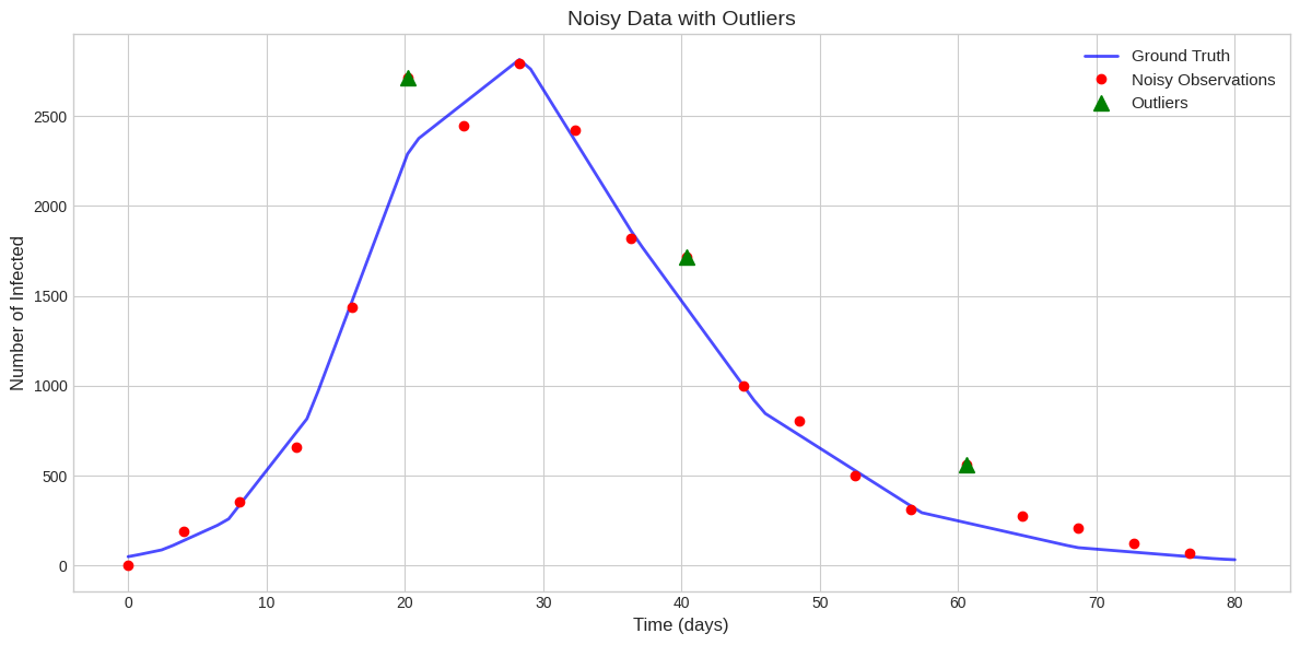
8. Practical Example: Handling Noisy and Missing Data

Real-world data often has noise, outliers, and missing observations.

8.1 Generate Realistic Noisy Data

# Generate data with more realistic noise
np.random.seed(123)

# Ground truth with more time points
ground_truth = SIR()
ground_truth(
    inits=[TOTAL_POPULATION - INITIAL_INFECTED, INITIAL_INFECTED, 0],
    trange=[0, 80],
    totpop=TOTAL_POPULATION,
    params={'beta': 0.35, 'gamma': 0.12},
)

# Create denser time points for sampling
full_times = np.linspace(0, 80, 100)
from scipy.interpolate import interp1d
interp_I = interp1d(ground_truth.traces['time'], ground_truth.traces['I'], kind='linear', fill_value='extrapolate')
full_I = interp_I(full_times)

# Sample every 5 days (realistic observation frequency)
sample_indices = np.arange(0, len(full_times), 5)
sample_times = full_times[sample_indices]
sample_I = full_I[sample_indices]

# Add noise with some outliers
noisy_I = sample_I + np.random.normal(0, 50, size=len(sample_I))

# Add a few outliers (indices within range)
n_samples = len(sample_times)
outlier_indices = [min(5, n_samples-1), min(10, n_samples-1), min(15, n_samples-1)]
outlier_indices = [i for i in outlier_indices if i < n_samples]
noisy_I[outlier_indices] += np.random.uniform(200, 400, size=len(outlier_indices))

# Ensure non-negative
noisy_I = np.maximum(noisy_I, 0)

print(f"Sampled {len(sample_times)} time points from {len(full_times)} total")
print(f"Added outliers at indices: {outlier_indices}")

Sampled 20 time points from 100 total
Added outliers at indices: [5, 10, 15]

# Plot the noisy data
fig, ax = plt.subplots(figsize=(12, 6))

ax.plot(full_times, full_I,
        'b-', label='Ground Truth', linewidth=2, alpha=0.7)
ax.plot(sample_times, noisy_I, 'ro', label='Noisy Observations', markersize=6)
if outlier_indices:
    ax.plot(sample_times[outlier_indices], noisy_I[outlier_indices],
            'g^', label='Outliers', markersize=10)

ax.set_xlabel('Time (days)', fontsize=12)
ax.set_ylabel('Number of Infected', fontsize=12)
ax.set_title('Noisy Data with Outliers', fontsize=14)
ax.legend(fontsize=11)
plt.tight_layout()
plt.show()

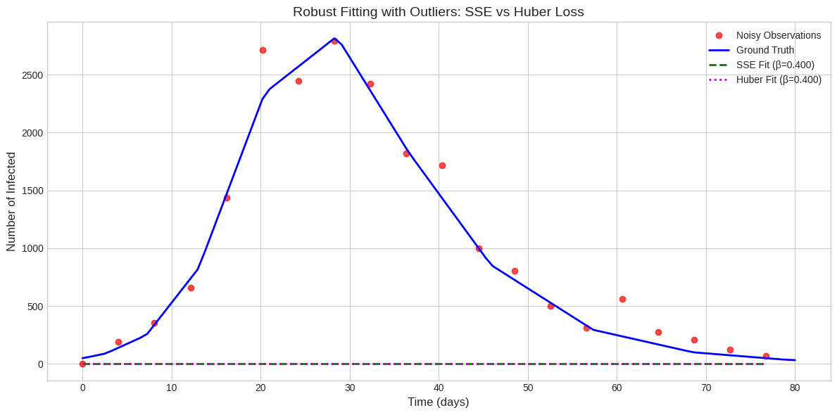
8.2 Compare SSE vs Huber Loss on Noisy Data

# Create dataset with noisy data
noisy_dataset = Dataset(SIR())
noisy_dataset.register(
    name='noisy_infected',
    values=noisy_I,
    times=sample_times,
    state_variable='I',
)

# Parameters to fit
noisy_params = [
    ParameterSpec(name='beta', bounds=(0.1, 0.8), initial=0.4),
    ParameterSpec(name='gamma', bounds=(0.05, 0.3), initial=0.15),
]

# Fit with SSE
fitter_sse = ModelFitter(
    model=SIR(),
    dataset=noisy_dataset,
    parameters_to_fit=noisy_params,
    total_population=TOTAL_POPULATION,
    loss_fn=SumOfSquaredErrors(),
)
result_sse = fitter_sse.fit()

# Fit with Huber loss (robust to outliers)
fitter_huber = ModelFitter(
    model=SIR(),
    dataset=noisy_dataset,
    parameters_to_fit=noisy_params,
    total_population=TOTAL_POPULATION,
    loss_fn=HuberLoss(delta=50.0),
)
result_huber = fitter_huber.fit()

print("Comparison on noisy data with outliers:")
print(f"  True:     beta=0.35, gamma=0.12")
print(f"  SSE:      beta={result_sse.best_params['beta']:.3f}, gamma={result_sse.best_params['gamma']:.3f}")
print(f"  Huber:    beta={result_huber.best_params['beta']:.3f}, gamma={result_huber.best_params['gamma']:.3f}")

Comparison on noisy data with outliers:
  True:     beta=0.35, gamma=0.12
  SSE:      beta=0.400, gamma=0.150
  Huber:    beta=0.400, gamma=0.150

# Visualize comparison
fig, ax = plt.subplots(figsize=(12, 6))

# Observations
ax.plot(sample_times, noisy_I, 'ro', label='Noisy Observations', markersize=6, alpha=0.7)

# Ground truth
ax.plot(full_times, full_I,
        'b-', label='Ground Truth', linewidth=2)

# SSE fit
if result_sse.fitted_model and result_sse.fitted_model.traces:
    ax.plot(result_sse.fitted_model.traces['time'], result_sse.fitted_model.traces['I'],
            'g--', label=f"SSE Fit (β={result_sse.best_params['beta']:.3f})", linewidth=2)

# Huber fit
if result_huber.fitted_model and result_huber.fitted_model.traces:
    ax.plot(result_huber.fitted_model.traces['time'], result_huber.fitted_model.traces['I'],
            'm:', label=f"Huber Fit (β={result_huber.best_params['beta']:.3f})", linewidth=2)

ax.set_xlabel('Time (days)', fontsize=12)
ax.set_ylabel('Number of Infected', fontsize=12)
ax.set_title('Robust Fitting with Outliers: SSE vs Huber Loss', fontsize=14)
ax.legend(fontsize=10)
plt.tight_layout()
plt.show()

9. Convenience Function

For quick fitting, use the fit_model convenience function.

# Quick fit with convenience function
result_quick = fit_model(
    model=SIR(),
    data={'I': observed_I},
    times=true_times,
    params_to_fit={'beta': (0.1, 1.0), 'gamma': (0.01, 0.5)},
    total_population=TOTAL_POPULATION,
    variable_mapping={'I': 'I'},
)

print("Quick fit results:")
print(f"  beta: {result_quick.best_params['beta']:.4f}")
print(f"  gamma: {result_quick.best_params['gamma']:.4f}")
print(f"  R0: {result_quick.best_params['beta'] / result_quick.best_params['gamma']:.2f}")

Quick fit results:
  beta: 0.4067
  gamma: 0.1008
  R0: 4.03

10. Summary and Best Practices

Key Takeaways

1. Data Registration: Always validate your dataset before fitting

2. Loss Functions: Choose based on your data type:

   • SSE for general use

   • Poisson/NegBinom for count data

   • Huber for data with outliers

3. Optimizers:

   • L-BFGS-B for fast, local optimization (good initial guess)

   • Differential evolution for global optimization

   • Multi-start for robustness

4. Parameter Scaling: Use log_scale=True for parameters spanning orders of magnitude

5. Validation: Use profile likelihood for confidence intervals

Common Pitfalls

• Poor initial guesses: Can lead to local minima

• Wrong loss function: SSE on count data can over-weight high values

• Too narrow bounds: May exclude true parameter values

• Ignoring validation: Data issues should be caught early

# Clean up
print("\n" + "="*60)
print("Tutorial complete!")
print("="*60)

============================================================
Tutorial complete!
============================================================