Phase Space Analysis Tools

This notebook demonstrates the phase space analysis tools in epimodels.tools.phase. These tools are based on nonlinear time series analysis techniques, particularly Takens’ embedding theorem.

Overview

• TimeDelayEmbedding: Class for phase space reconstruction

• phase_portrait: Create 2D phase portraits

• find_optimal_embedding: Automatically find optimal parameters

import numpy as np
import matplotlib.pyplot as plt
from epimodels.continuous import SIR, SEIR
from epimodels.tools.phase import (
    TimeDelayEmbedding,
    phase_portrait,
    find_optimal_embedding,
)

%matplotlib inline

1. Basic Phase Portraits

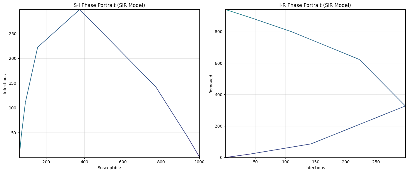
A phase portrait shows the trajectory of a dynamical system in phase space. For epidemic models, we can plot any two state variables against each other.

# Run an SIR model
model = SIR()
model([1000, 1, 0], [0, 250], 1001, {'beta': 0.3, 'gamma': 0.1})

print(f"R0 = {model.R0:.2f}")

R0 = 3.00

# Create phase portrait of S vs I
fig, axes = plt.subplots(1, 2, figsize=(14, 6))

# S vs I phase portrait
phase_portrait(
    model.traces['S'],
    model.traces['I'],
    ax=axes[0],
    color_by_time=True
)
axes[0].set_xlabel('Susceptible')
axes[0].set_ylabel('Infectious')
axes[0].set_title('S-I Phase Portrait (SIR Model)')

# I vs R phase portrait
phase_portrait(
    model.traces['I'],
    model.traces['R'],
    ax=axes[1],
    color_by_time=True
)
axes[1].set_xlabel('Infectious')
axes[1].set_ylabel('Removed')
axes[1].set_title('I-R Phase Portrait (SIR Model)')

plt.tight_layout()

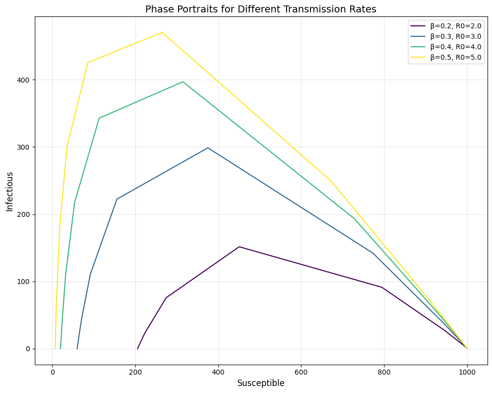
Multiple Trajectories

Compare phase portraits for different parameter values.

fig, ax = plt.subplots(figsize=(10, 8))

betas = [0.2, 0.3, 0.4, 0.5]
colors = plt.cm.viridis(np.linspace(0, 1, len(betas)))

for beta, color in zip(betas, colors):
    model = SIR()
    model([1000, 1, 0], [0, 200], 1001, {'beta': beta, 'gamma': 0.1})
    ax.plot(model.traces['S'], model.traces['I'],
            color=color, linewidth=1.5, label=f'β={beta}, R0={beta/0.1:.1f}')

ax.set_xlabel('Susceptible', fontsize=12)
ax.set_ylabel('Infectious', fontsize=12)
ax.set_title('Phase Portraits for Different Transmission Rates', fontsize=14)
ax.legend()
ax.grid(True, alpha=0.3)
plt.tight_layout()

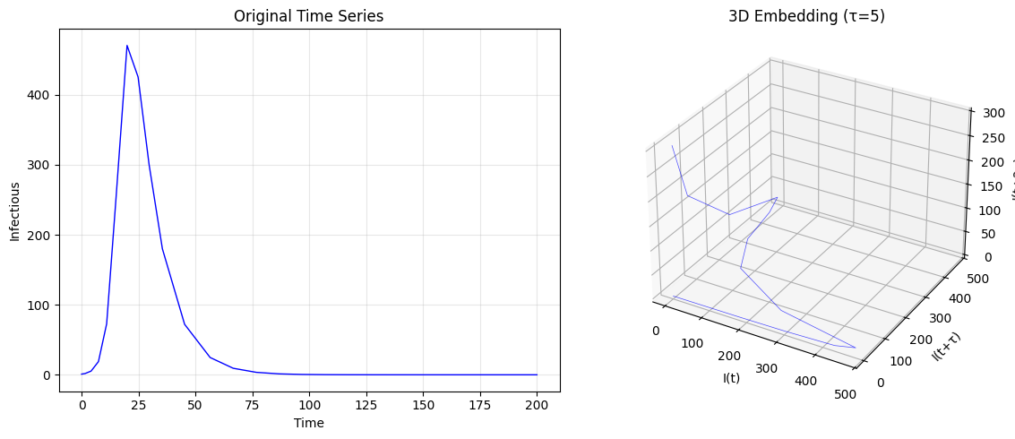
2. Time Delay Embedding

Time delay embedding reconstructs the phase space from a single time series using Takens’ theorem. This is useful for analyzing the dynamics when you only observe one variable.

The Embedding

Given a time series \(x(t)\), we create embedded vectors:

\[\vec{y}(t) = [x(t), x(t+\tau), x(t+2\tau), ..., x(t+(d-1)\tau)]\]

where:

• \(\tau\) is the time delay

• \(d\) is the embedding dimension

# Get the infectious time series from our model
I = model.traces['I']
time = model.traces['time']

# Create embedding with tau=5 and dimension=3
embedding = TimeDelayEmbedding(I, tau=5, dim=3)
embedded = embedding.embed()

print(f"Original time series length: {len(I)}")
print(f"Embedded data shape: {embedded.shape}")

Original time series length: 28
Embedded data shape: (18, 3)

# Visualize the embedded trajectory in 3D
from mpl_toolkits.mplot3d import Axes3D

fig = plt.figure(figsize=(12, 5))

# Original time series
ax1 = fig.add_subplot(121)
ax1.plot(time, I, 'b-', linewidth=1)
ax1.set_xlabel('Time')
ax1.set_ylabel('Infectious')
ax1.set_title('Original Time Series')
ax1.grid(True, alpha=0.3)

# 3D embedding
ax2 = fig.add_subplot(122, projection='3d')
ax2.plot(embedded[:, 0], embedded[:, 1], embedded[:, 2],
         'b-', linewidth=0.5, alpha=0.7)
ax2.set_xlabel('I(t)')
ax2.set_ylabel('I(t+τ)')
ax2.set_zlabel('I(t+2τ)')
ax2.set_title('3D Embedding (τ=5)')

plt.tight_layout()

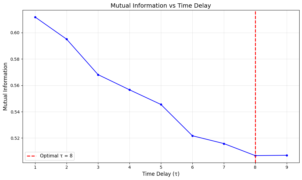
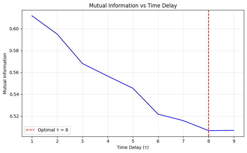
3. Finding Optimal Time Delay (τ)

The mutual information method helps find the optimal time delay. The first local minimum of mutual information is a good choice for τ.

# Run a model to get time series
model = SIR()
model([1000, 1, 0], [0, 500], 1001, {'beta': 0.3, 'gamma': 0.1}, t_eval=range(0, 500))

# Find optimal tau using mutual information
embedding = TimeDelayEmbedding(model.traces['I'])
tau_opt, mi_values = embedding.mutual_information(tau_max=30)

print(f"Optimal time delay (τ): {tau_opt}")

Optimal time delay (τ): 8

# Plot mutual information
fig, ax = plt.subplots(figsize=(10, 6))

taus = range(1, len(mi_values) + 1)
ax.plot(taus, mi_values, 'b-o', linewidth=1.5, markersize=4)
ax.axvline(tau_opt, color='r', linestyle='--', linewidth=2,
           label=f'Optimal τ = {tau_opt}')

ax.set_xlabel('Time Delay (τ)', fontsize=12)
ax.set_ylabel('Mutual Information', fontsize=12)
ax.set_title('Mutual Information vs Time Delay', fontsize=14)
ax.legend(fontsize=11)
ax.grid(True, alpha=0.3)
plt.tight_layout()

Using the built-in plot method

# Alternative: use the built-in plotting method
embedding = TimeDelayEmbedding(model.traces['I'])
ax = embedding.plot_mutual_information(tau_max=30)
plt.tight_layout()

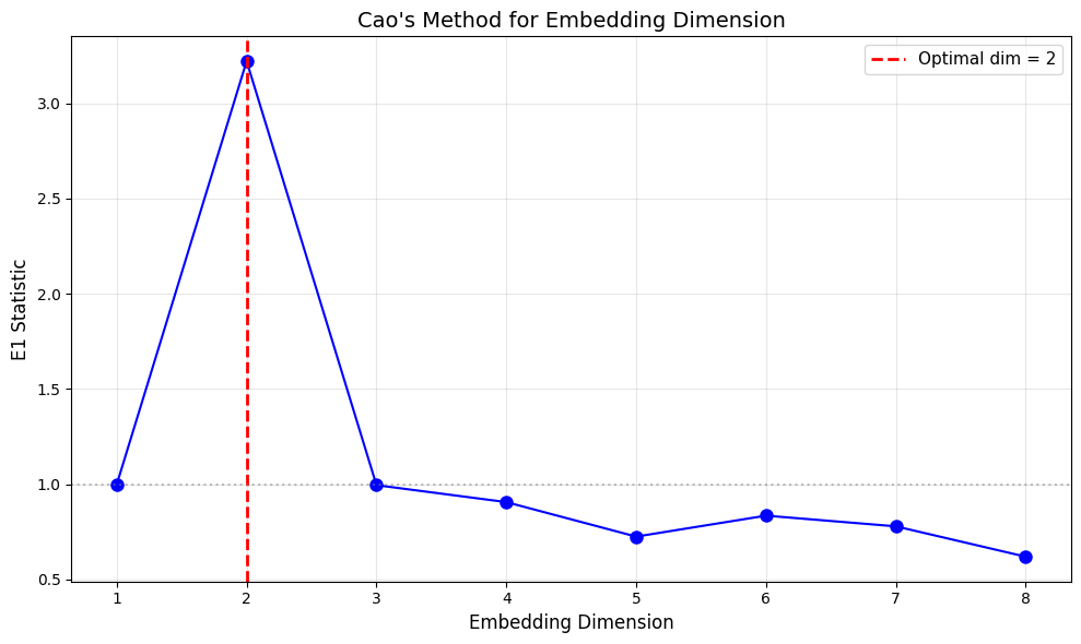
4. Finding Optimal Embedding Dimension

Cao’s method uses the E1 statistic to determine the minimum embedding dimension. When E1 saturates (stops increasing), the corresponding dimension is sufficient.

# Find optimal embedding dimension
embedding = TimeDelayEmbedding(model.traces['I'], tau=tau_opt)
dim_opt, e1_values = embedding.cao_embedding_dimension(dim_max=8)

print(f"Optimal embedding dimension: {dim_opt}")

Optimal embedding dimension: 2

# Plot E1 statistic
fig, ax = plt.subplots(figsize=(10, 6))

dims = range(1, len(e1_values) + 1)
ax.plot(dims, e1_values, 'b-o', linewidth=1.5, markersize=8)
ax.axvline(dim_opt, color='r', linestyle='--', linewidth=2,
           label=f'Optimal dim = {dim_opt}')
ax.axhline(1.0, color='gray', linestyle=':', alpha=0.5)

ax.set_xlabel('Embedding Dimension', fontsize=12)
ax.set_ylabel('E1 Statistic', fontsize=12)
ax.set_title('Cao\'s Method for Embedding Dimension', fontsize=14)
ax.legend(fontsize=11)
ax.grid(True, alpha=0.3)
ax.set_xticks(dims)
plt.tight_layout()

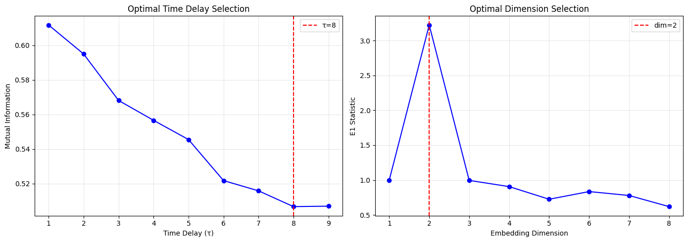
5. Automatic Parameter Selection

The find_optimal_embedding function combines both methods to automatically find optimal parameters.

# Find optimal embedding parameters automatically
params = find_optimal_embedding(
    model.traces['I'],
    tau_max=30,
    dim_max=8
)

print(f"Optimal τ: {params['tau']}")
print(f"Optimal dimension: {params['dim']}")

Optimal τ: 8
Optimal dimension: 2

# Visualize both analyses
fig, axes = plt.subplots(1, 2, figsize=(14, 5))

# Mutual information
axes[0].plot(range(1, len(params['mi_values'])+1), params['mi_values'], 'b-o')
axes[0].axvline(params['tau'], color='r', linestyle='--', label=f"τ={params['tau']}")
axes[0].set_xlabel('Time Delay (τ)')
axes[0].set_ylabel('Mutual Information')
axes[0].set_title('Optimal Time Delay Selection')
axes[0].legend()
axes[0].grid(True, alpha=0.3)

# Embedding dimension
axes[1].plot(range(1, len(params['e1_values'])+1), params['e1_values'], 'b-o')
axes[1].axvline(params['dim'], color='r', linestyle='--', label=f"dim={params['dim']}")
axes[1].set_xlabel('Embedding Dimension')
axes[1].set_ylabel('E1 Statistic')
axes[1].set_title('Optimal Dimension Selection')
axes[1].legend()
axes[1].grid(True, alpha=0.3)

plt.tight_layout()

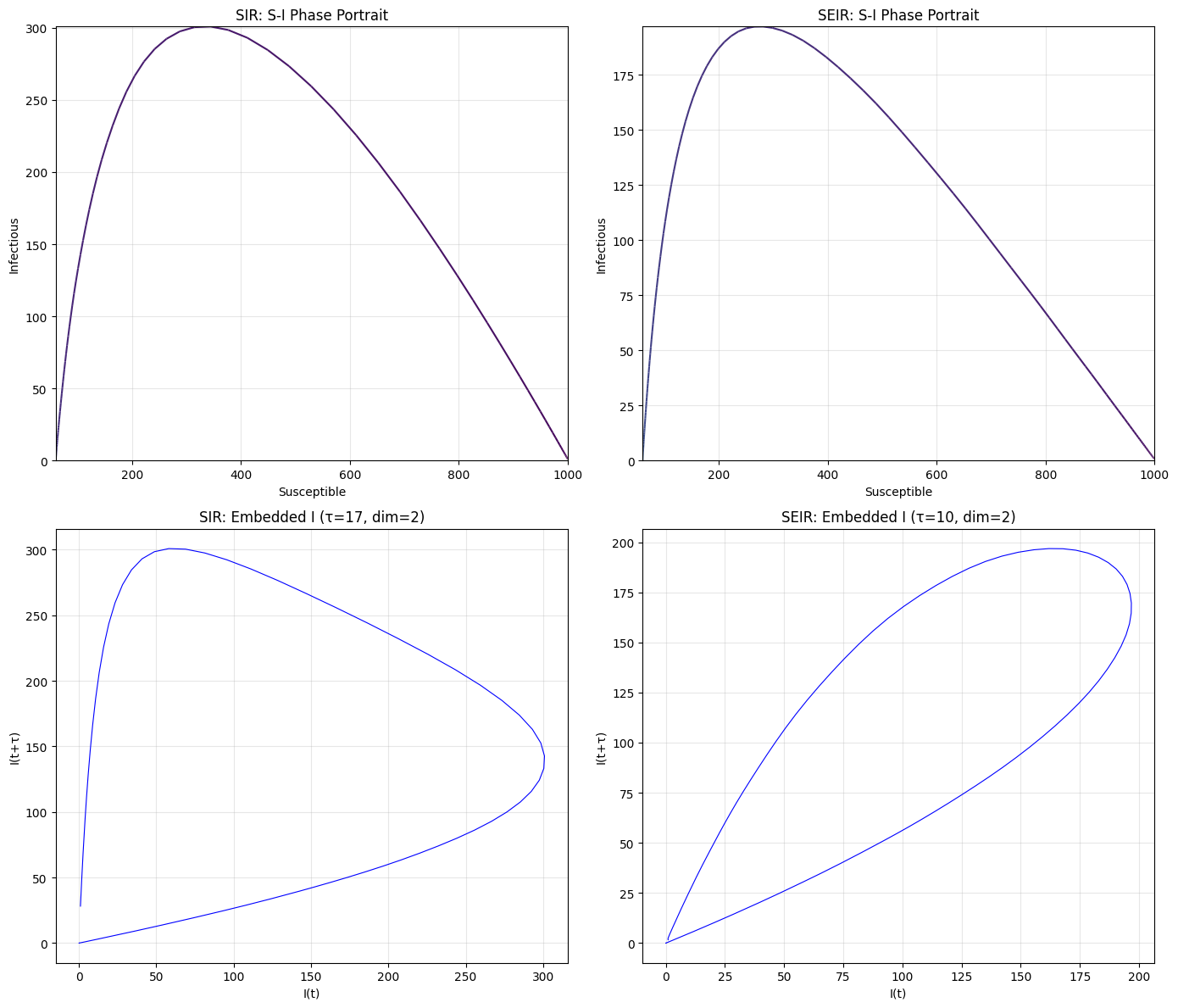
6. Comparing Different Epidemic Dynamics

Let’s compare the phase space characteristics of SIR and SEIR models.

# Run SIR model
sir = SIR()
sir([1000, 1, 0], [0, 550], 1001, {'beta': 0.3, 'gamma': 0.1}, t_eval=range(0, 550))

# Run SEIR model
seir = SEIR()
seir([1000, 0, 1, 0], [0, 550], 1001, {'beta': 0.3, 'gamma': 0.1, 'epsilon': 0.2}, t_eval=range(0, 550))

# Compare phase portraits
fig, axes = plt.subplots(2, 2, figsize=(14, 12))

# SIR: S vs I
phase_portrait(sir.traces['S'], sir.traces['I'], ax=axes[0, 0], color_by_time=True)
axes[0, 0].set_title('SIR: S-I Phase Portrait')
axes[0, 0].set_xlabel('Susceptible')
axes[0, 0].set_ylabel('Infectious')

# SEIR: S vs I
phase_portrait(seir.traces['S'], seir.traces['I'], ax=axes[0, 1], color_by_time=True)
axes[0, 1].set_title('SEIR: S-I Phase Portrait')
axes[0, 1].set_xlabel('Susceptible')
axes[0, 1].set_ylabel('Infectious')

# SIR: I embedded
sir_params = find_optimal_embedding(sir.traces['I'], tau_max=20, dim_max=6)
sir_emb = TimeDelayEmbedding(sir.traces['I'], tau=sir_params['tau'], dim=2).embed()
axes[1, 0].plot(sir_emb[:, 0], sir_emb[:, 1], 'b-', linewidth=0.8)
axes[1, 0].set_title(f'SIR: Embedded I (τ={sir_params["tau"]}, dim=2)')
axes[1, 0].set_xlabel('I(t)')
axes[1, 0].set_ylabel('I(t+τ)')
axes[1, 0].grid(True, alpha=0.3)

# SEIR: I embedded
seir_params = find_optimal_embedding(seir.traces['I'], tau_max=20, dim_max=6)
seir_emb = TimeDelayEmbedding(seir.traces['I'], tau=seir_params['tau'], dim=2).embed()
axes[1, 1].plot(seir_emb[:, 0], seir_emb[:, 1], 'b-', linewidth=0.8)
axes[1, 1].set_title(f'SEIR: Embedded I (τ={seir_params["tau"]}, dim=2)')
axes[1, 1].set_xlabel('I(t)')
axes[1, 1].set_ylabel('I(t+τ)')
axes[1, 1].grid(True, alpha=0.3)

plt.tight_layout()

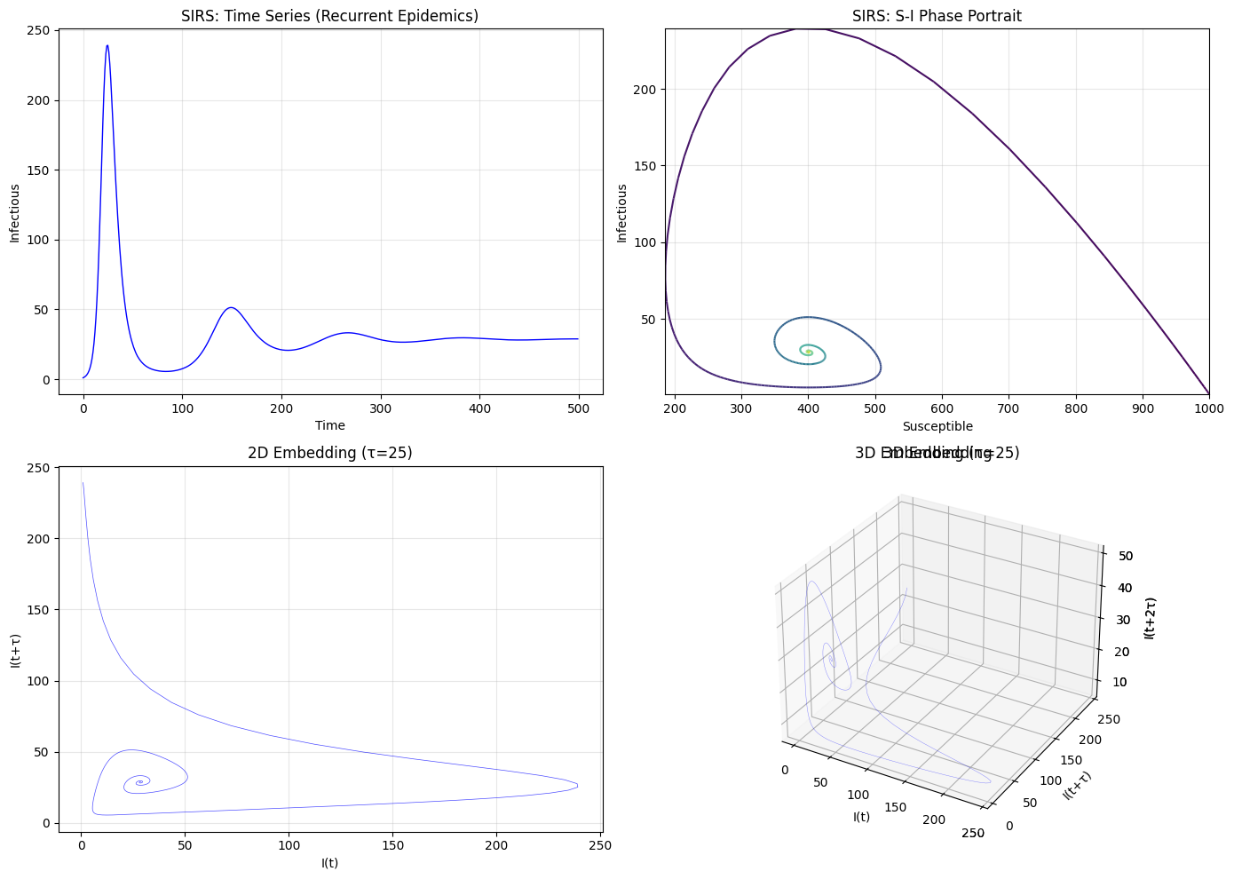
7. Analyzing Recurrent Epidemics (SIRS Model)

The SIRS model exhibits recurrent epidemics due to waning immunity. Let’s analyze its phase space.

from epimodels.continuous import SIRS

# Run SIRS model with waning immunity
sirs = SIRS()
sirs([1000, 1, 0], [0, 500], 1001, {'beta': 0.5, 'gamma': 0.2, 'xi': 0.01}, t_eval=range(0, 500))

print(f"R0 = {sirs.R0:.2f}")

R0 = 2.50

fig, axes = plt.subplots(2, 2, figsize=(14, 10))

# Time series
axes[0, 0].plot(sirs.traces['time'], sirs.traces['I'], 'b-', linewidth=1)
axes[0, 0].set_xlabel('Time')
axes[0, 0].set_ylabel('Infectious')
axes[0, 0].set_title('SIRS: Time Series (Recurrent Epidemics)')
axes[0, 0].grid(True, alpha=0.3)

# Phase portrait
phase_portrait(sirs.traces['S'], sirs.traces['I'], ax=axes[0, 1], color_by_time=True)
axes[0, 1].set_title('SIRS: S-I Phase Portrait')
axes[0, 1].set_xlabel('Susceptible')
axes[0, 1].set_ylabel('Infectious')

# Find optimal embedding
params = find_optimal_embedding(sirs.traces['I'], tau_max=30, dim_max=6)
print(f"\nOptimal embedding parameters:")
print(f"  τ = {params['tau']}")
print(f"  dim = {params['dim']}")

# 2D embedding
embedded = TimeDelayEmbedding(sirs.traces['I'], tau=params['tau'], dim=2).embed()
axes[1, 0].plot(embedded[:, 0], embedded[:, 1], 'b-', linewidth=0.5, alpha=0.7)
axes[1, 0].set_title(f'2D Embedding (τ={params["tau"]})')
axes[1, 0].set_xlabel('I(t)')
axes[1, 0].set_ylabel('I(t+τ)')
axes[1, 0].grid(True, alpha=0.3)

# 3D embedding
embedded_3d = TimeDelayEmbedding(sirs.traces['I'], tau=params['tau'], dim=3).embed()
ax3d = fig.add_subplot(2, 2, 4, projection='3d')
ax3d.plot(embedded_3d[:, 0], embedded_3d[:, 1], embedded_3d[:, 2],
          'b-', linewidth=0.3, alpha=0.5)
ax3d.set_xlabel('I(t)')
ax3d.set_ylabel('I(t+τ)')
ax3d.set_zlabel('I(t+2τ)')
ax3d.set_title(f'3D Embedding')

# Redraw the 3D plot in the correct position
axes[1, 1].remove()
ax3d = fig.add_subplot(2, 2, 4, projection='3d')
ax3d.plot(embedded_3d[:, 0], embedded_3d[:, 1], embedded_3d[:, 2],
          'b-', linewidth=0.3, alpha=0.5)
ax3d.set_xlabel('I(t)')
ax3d.set_ylabel('I(t+τ)')
ax3d.set_zlabel('I(t+2τ)')
ax3d.set_title(f'3D Embedding (τ={params["tau"]})')

plt.tight_layout()

Optimal embedding parameters:
  τ = 25
  dim = 2

Summary

The epimodels.tools.phase module provides tools for:

1. Phase Portraits: Visualize system dynamics in phase space

2. Time Delay Embedding: Reconstruct phase space from single time series

3. Parameter Selection: Automatically find optimal τ and dimension

Key Functions

Function/Class	Purpose
TimeDelayEmbedding	Create embedded vectors from time series
phase_portrait()	Plot 2D phase portraits
find_optimal_embedding()	Find optimal τ and dimension

References

1. Takens, F. (1981). Detecting strange attractors in turbulence.

2. Cao, L. (1997). Practical method for determining the minimum embedding dimension.

3. Basharat, A., & Shah, M. (2009). Time series prediction by chaotic modeling.