Simulating Continuous models¶

[1]:

from epimodels.continuous import models as CM

[2]:

from IPython.display import Markdown as md
import numpy as np
import matplotlib.pyplot as P

First we instantiate the model type we want to use. The representation of the model is a \(\LaTeX\) expression of the model. This can be useful when writing a Document in \(\LaTeX\) about your work.

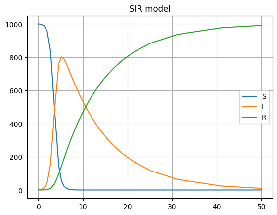
SIR model¶

The SIR (Susceptible-Infectious-Removed) model is a classic compartmental model for infectious disease dynamics.

[3]:

model = CM.SIR()
md(str(model))

[3]:

Model: SIR¶

flowchart LR

S(Susceptible) -->|$$\beta$$| I(Infectious)
I -->|$$\gamma$$| R(Removed)

[4]:

model([1000, 1, 0], [0, 50], 1001, {'beta': 2, 'gamma': .1})
model.plot_traces()

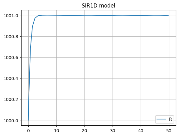
../_images/Examples_Continuous_models_6_0.png

SIR1D¶

The SIR1D model is a variant of the SIR model that includes a dimensionless parameter \(\xi\) that controls the rate of recovery.

[5]:

model = CM.SIR1D()
md(str(model))

[5]:

Model: SIR1D¶

flowchart LR

S(Susceptible) -->|$$\beta$$| I(Infectious)
I -->|$$\gamma$$| R(Recovered)

[6]:

model([1000, 1], [0, 50], 1001, {'R0': 1.5,'gamma':1.5, 'S0':1000})
model.plot_traces()

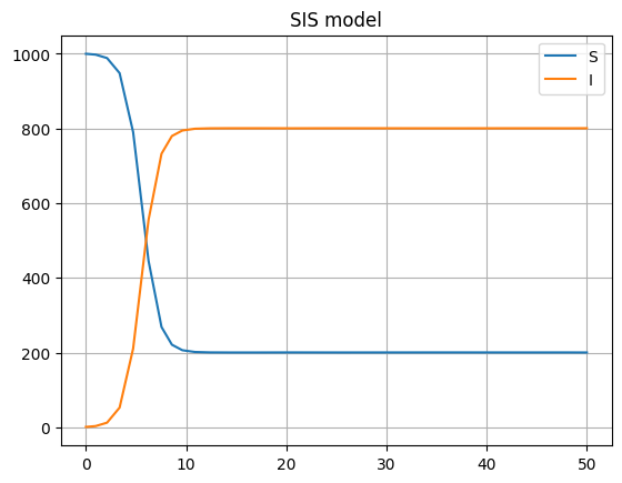
../_images/Examples_Continuous_models_9_0.png

SIS model¶

The SIS (Susceptible-Infectious-Susceptible) model is used for diseases that do not confer immunity after recovery.

[7]:

model = CM.SIS()
md(str(model))

[7]:

Model: SIS¶

flowchart LR

S(Susceptible) -->|$$\beta$$| I(Infectious)
I -->|$$\gamma$$| S

[8]:

model([1000, 1], [0, 50], 1001, {'beta': 1.5, 'gamma': 0.3})
model.plot_traces()

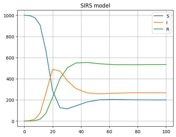
../_images/Examples_Continuous_models_12_0.png

SIRS model¶

The SIRS (Susceptible-Infectious-Removed-Susceptible) model accounts for waning immunity over time.

[9]:

model = CM.SIRS()
md(str(model))

[9]:

Model: SIRS¶

flowchart LR

S(Susceptible) -->|$$\beta$$| I(Infectious)
I -->|$$\gamma$$| R(Removed)
R -->|$$\xi$$| S

[10]:

model([1000, 1, 0], [0, 100], 1001, {'beta': 0.5, 'gamma': 0.1, 'xi': 0.05})
model.plot_traces()

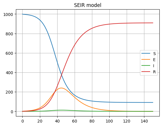
../_images/Examples_Continuous_models_15_0.png

SEIR model¶

The SEIR (Susceptible-Exposed-Infectious-Removed) model includes an exposed compartment for diseases with an incubation period.

[11]:

model = CM.SEIR()
md(str(model))

[11]:

Model: SEIR¶

flowchart LR

S(Susceptible) -->|$$\beta$$| E(Exposed)
E -->|$$\epsilon$$| I(Infectious)
I -->|$$\gamma$$| R(Removed)

[12]:

model([1000, 0, 1, 0], [0, 150], 1001, {'beta': 5, 'gamma': 1.9, 'epsilon': 0.1})
model.plot_traces()

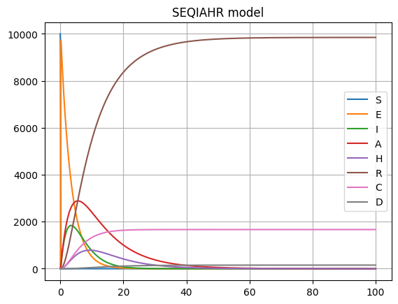
../_images/Examples_Continuous_models_18_0.png

SEQIAHR model¶

The SEQIAHR model is a more complex compartmental model that includes asymptomatic and hospitalized compartments, suitable for modeling diseases like COVID-19.

[13]:

model = CM.SEQIAHR()
md(str(model))

[13]:

Model: SEQIAHR¶

flowchart LR

S(Susceptible) -->|$$\beta$$| E(Exposed)
E -->|"$$\alpha(1-p)$$"| I(Infectious)
E -->|$$\alpha p$$| A(Asymptomatic)
I -->|$$\phi$$| H(Hospitalized)
I -->|$$\delta$$| R(Removed)
A -->|$$\gamma$$| R
H -->|$$\rho$$| R
H -->|$$\mu$$| D(Deaths)

[14]:

params = {
    'chi': 0.3,    # Quarantine reduction factor
    'phi': 0.1,    # Hospitalization rate from I
    'beta': 0.5,   # Transmission rate
    'rho': 0.1,    # Recovery rate from H
    'delta': 0.2,  # Recovery rate from I
    'gamma': 0.1,  # Recovery rate from A
    'alpha': 0.3,  # Incubation rate
    'mu': 0.01,    # Mortality rate in H
    'p': 0.5,      # Proportion asymptomatic
    'q': 20,       # Quarantine start day
    'r': 30        # Quarantine duration
}
inits = [10000, 0, 1, 0, 0, 0, 0, 0]
model(inits, [0, 100], 10001, params)
model.plot_traces()

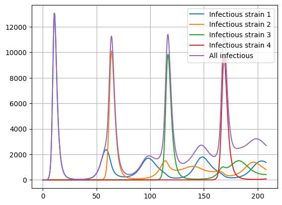
../_images/Examples_Continuous_models_21_0.png

Dengue 4-strain model¶

A complex model for dengue fever with four serotypes, accounting for cross-immunity and antibody-dependent enhancement.

[15]:

model = CM.Dengue4Strain()
md(str(model))

[15]:

Model: Dengue4Strain¶

flowchart LR
    S(Susceptible) -->|$$\beta$$| I1(I 1)
    S -->|$$\beta$$| I2(I 2)
    S -->|$$\beta$$| I3(I 3)
    S -->|$$\beta$$| I4(I 4)

    I1 -->|$$\sigma$$| R1(R 1)
    I2 -->|$$\sigma$$| R2(R 2)
    I3 -->|$$\sigma$$| R3(R 3)
    I4 -->|$$\sigma$$| R4(R 4)

    R1 -->|$$\delta$$| I12(I 1+2)
    R1 -->|$$\delta$$| I13(I 1+3)
    R1 -->|$$\delta$$| I14(I 1+4)

    R2 -->|$$\delta$$| I21(I 2+1)
    R2 -->|$$\delta$$| I23(I 2+3)
    R2 -->|$$\delta$$| I24(I 2+4)

    R3 -->|$$\delta$$| I31(I 3+1)
    R3 -->|$$\delta$$| I32(I 3+2)
    R3 -->|$$\delta$$| I34(I 3+4)

    R4 -->|$$\delta$$| I41(I 4+1)
    R4 -->|$$\delta$$| I42(I 4+2)
    R4 -->|$$\delta$$| I43(I 4+3)

    I12 -->|$$\sigma$$| R12(R 1+2)
    I13 -->|$$\sigma$$| R13(R 1+3)
    I14 -->|$$\sigma$$| R14(R 1+4)

    I21 -->|$$\sigma$$| R12(R 1+2)
    I23 -->|$$\sigma$$| R23(R 2+3)
    I24 -->|$$\sigma$$| R24(R 2+4)

    I31 -->|$$\sigma$$| R13(R 1+3)
    I32 -->|$$\sigma$$| R23(R 2+3)
    I34 -->|$$\sigma$$| R34(R 3+4)

    I41 -->|$$\sigma$$| R14(R 1+4)
    I42 -->|$$\sigma$$| R24(R 2+4)
    I43 -->|$$\sigma$$| R34(R 3+4)

    R12 -->|$$\delta$$| I123(I 1+2+3)
    R13 -->|$$\delta$$| I132(I 1+3+2)
    R14 -->|$$\delta$$| I142(I 1+4+2)

    R12 -->|$$\delta$$| I213(I 2+1+3)
    R23 -->|$$\delta$$| I231(I 2+3+1)
    R24 -->|$$\delta$$| I241(I 2+4+1)

    R24 -->|$$\delta$$| I243(I 2+4+3)
    R34 -->|$$\delta$$| I341(I 3+4+1)
    R34 -->|$$\delta$$| I342(I 3+4+2)

    R23 -->|$$\delta$$| I234(I 2+3+4)
    R14 -->|$$\delta$$| I143(I 1+4+3)
    R13 -->|$$\delta$$| I134(I 1+3+4)

    R12 -->|$$\delta$$| I124(I 1+2+4)

    I123 -->|$$\sigma$$| R123(R 1+2+3)
    I132 -->|$$\sigma$$| R123(R 1+2+3)
    I124 -->|$$\sigma$$| R124(R 1+2+4)

    I142 -->|$$\sigma$$| R124(R 1+2+4)
    I143 -->|$$\sigma$$| R134(R 1+3+4)
    I134 -->|$$\sigma$$| R134(R 1+3+4)

    I234 -->|$$\sigma$$| R234(R 2+3+4)
    I243 -->|$$\sigma$$| R234(R 2+3+4)
    I341 -->|$$\sigma$$| R134(R 1+3+4)

    I342 -->|$$\sigma$$| R234(R 2+3+4)
    I231 -->|$$\sigma$$| R123(R 1+2+3)
    I241 -->|$$\sigma$$| R124(R 1+2+4)

    R123 -->|$$\delta$$| I1234(I 1+2+3+4)
    R124 -->|$$\delta$$| I1243(I 1+2+4+3)
    R134 -->|$$\delta$$| I1342(I 1+3+4+2)
    R234 -->|$$\delta$$| I2341(I 2+3+4+1)

    I1234 -->|$$\sigma$$| R1234(R 1+2+3+4)
    I1243 -->|$$\sigma$$| R1234(R 1+2+3+4)
    I1342 -->|$$\sigma$$| R1234(R 1+2+3+4)
    I2341 -->|$$\sigma$$| R1234(R 1+2+3+4)

    classDef strain1 fill:#ffcccc,stroke:#ff0000
    classDef strain2 fill:#ccffcc,stroke:#00ff00
    classDef strain3 fill:#ccccff,stroke:#0000ff
    classDef strain4 fill:#ffccff,stroke:#ff00ff

    class I1,I21,I31,I41,I231,I241,I341,I2341 strain1
    class I2,I12,I32,I42,I132,I213,I342,I142,I1342 strain2
    class I3,I13,I23,I43,I123,I143,I243,I1243 strain3
    class I4,I14,I24,I34,I142,I124,I134,I342,I124,I134,I234,I1234 strain4;

[16]:

inits = [48000, 0, 0, 0, 0, 0, 0, 0, 0, 0, 0, 0, 0, 0, 0, 0, 0, 0, 0, 0, 0, 0, 0, 0, 0, 0, 0, 0, 0,
             0, 0, 0, 0, 0, 0, 0, 0, 0, 0, 0, 0, 0, 0, 0, 0, 0, 0, 0]
pars = {
    'beta': 100 / (50000 * 52),  # 200 novos casos per capita per year
    'N': 50000, #population size
    'delta': 0.79,  # Cross-immunity protection. 1 means no cross-immunity
    'mu': 1 / (1 * 52),  # natural Birth/Mortality rate
    'sigma': 1 / 1.5,  # recovery rate
    'im': [1, 52, 104, 156] #  Week of arrival of cases for each strain
}
model(inits, [0, 208], 50000, pars, max_step=0.1)

[17]:

pts = len(model.traces['time'])
Ia1 = np.zeros(pts) # All infectious for strain 1
Ia2 = np.zeros(pts) # All infectious for strain 2
Ia3 = np.zeros(pts) # All infectious for strain 3
Ia4 = np.zeros(pts) # All infectious for strain 4
Iall = np.zeros(pts)
for v,tr in model.traces.items():
    if not v.startswith('I_'):
        continue
    Iall += tr
    if v.endswith('1'):
        Ia1 += tr
    elif v.endswith('2'):
        Ia2 += tr
    elif v.endswith('3'):
        Ia3 += tr
    elif v.endswith('4'):
        Ia4 += tr

P.plot(model.traces['time'], Ia1, label='Infectious strain 1')
P.plot(model.traces['time'], Ia2, label='Infectious strain 2')
P.plot(model.traces['time'], Ia3, label='Infectious strain 3')
P.plot(model.traces['time'], Ia4, label='Infectious strain 4')
P.plot(model.traces['time'], Iall, label='All infectious')
P.grid()
P.legend(loc=0);

../_images/Examples_Continuous_models_25_0.png

SIR-SEI model¶

[ ]:

climate_params = {
"T_prime": 21.6,

"T1": 26.4,
"T2": 0.025,
"omega1": 0.017,
"phi1": 1.45,

"R1": 250.083,
"R2": 0.565,
"omega2": 0.02,
"phi2": 1.6,
}

mosquito_params = {
"BE": 200,
"pME": 0.9,
"pML": 0.25,
"pMP": 0.75,
"tauE": 1,
"tauP": 1,
"c1": 0.0554,
"c2": 0.1737,
"D1": 32.5,
"RL": 32.26,
}

transmission_params = {
"b1": 0.4,
"b2": 0.7,
"A": 32.5,
"B": 15,
"C": 48.78,
}

human_params = {
"mu_H": 0.00004,
"gamma": 1/120,
"tau_H": 10,
}

development_params = {
"DD": 105,
"Tmin": 14.5,
}

population_params = {
"N": 9586,
"M": 3000
}

[ ]:

params = {
**climate_params,
**mosquito_params,
**transmission_params,
**human_params,
**development_params,
**population_params
}

[ ]:

E_M0 = 10
I_M0 = 0
I_H0 = 1000
R_H0 = 100

N = params["N"]
M = params["M"]

S_H0 = N - I_H0 - R_H0
S_M0 = M - E_M0 - I_M0

inits = [
S_H0,
I_H0,
R_H0,
S_M0,
E_M0,
I_M0
]

[ ]:

model = CM.SIRSEI()

md(str(model))

model(
    inits,
    [0, 1825],
    12586,
    params
)


model.plot(compartments=['Sh', 'Ih', 'Rh'])
model.plot(compartments=['Sv', 'Ev', 'Iv'])